LeR Advanced Sampling — Generating Detectable Events
This notebook is created by Phurailatpam Hemantakumar
This notebook demonstrates how to generate a specific number of detectable events and monitor detection rate convergence as a function of sample size using the LeR class.
Key Features:
Batch sampling until N detectable events are collected
Rate convergence monitoring with stopping criteria
Resume capability for interrupted sessions
Visualization of rate convergence and parameter distributions
Table of Contents
Initialize LeR
Sampling N Detectable Events
2.1 Unlensed Events
2.2 Rate Convergence (Unlensed)
2.3 Rate Stability (Unlensed)
2.4 Lensed Events
2.5 Rate Convergence (Lensed)
2.6 Rate Stability (Lensed)
2.7 Rate Comparison
Parameter Distributions: All vs Detectable
3.1 Unlensed Events
3.2 Lensed Events
Visualizing Lensed Detectable Events
4.1 Redshift Distribution
4.2 Magnification Ratio vs Time Delay
4.3 Caustic Plot
Summary
1. Initialize LeR
The LeR class is the main interface for simulating unlensed and lensed GW events and calculating detection rates. Default settings:
Event type: BBH (Binary Black Hole)
Lens model: EPL+Shear (Elliptical Power Law with external shear)
Detectors: H1, L1, V1 with O4 design sensitivity
Outputs are saved to ./ler_data by default.
[1]:
# Import LeR
from ler.rates import LeR

# Initialize LeR with default settings
# npool: number of parallel processes for sampling
# use this gwsnr's input args if you want SNR values in the output, besides the boolean detection probability values. This will increase the output dictionary size and the runtime of the code. For details, refer to https://gwsnr.hemantaph.com/examples/pdet_generation.html.:
# pdet_kwargs=dict(snr_th=10.0, snr_th_net=10.0, pdet_type="boolean", distribution_type="noncentral_chi2", include_optimal_snr=True, include_observed_snr=True)
ler = LeR(npool=6)
Initializing LeR class...


Initializing LensGalaxyParameterDistribution class...


Initializing OpticalDepth class

comoving_distance interpolator will be loaded from ./interpolator_json/comoving_distance/comoving_distance_0.json
angular_diameter_distance interpolator will be loaded from ./interpolator_json/angular_diameter_distance/angular_diameter_distance_0.json
angular_diameter_distance interpolator will be loaded from ./interpolator_json/angular_diameter_distance/angular_diameter_distance_0.json
differential_comoving_volume interpolator will be loaded from ./interpolator_json/differential_comoving_volume/differential_comoving_volume_0.json
using ler available velocity dispersion function : velocity_dispersion_ewoud
velocity_dispersion_ewoud interpolator will be loaded from ./interpolator_json/velocity_dispersion/velocity_dispersion_ewoud_0.json
using ler available axis_ratio function : rayleigh
rayleigh interpolator will be loaded from ./interpolator_json/axis_ratio/rayleigh_0.json
using ler available axis_rotation_angle function : uniform
using ler available density_profile_slope function : normal
using ler available external_shear1 function : normal
using ler available external_shear2 function : normal
using ler available cross_section function : cross_section_epl_shear_njit
using ler available lens_redshift_sl function : lens_redshift_strongly_lensed_numerical
Numerically solving the lens redshift distribution...
lens_redshift_strongly_lensed_numerical interpolator will be loaded from ./interpolator_json/lens_redshift_sl/lens_redshift_strongly_lensed_numerical_0.json
using ler available lens_redshift function : lens_redshift_intrinsic_numerical
lens_redshift_intrinsic_numerical interpolator will be loaded from ./interpolator_json/lens_redshift/lens_redshift_intrinsic_numerical_1.json
using ler available optical depth function : optical_depth_numerical
optical_depth_numerical interpolator will be loaded from ./interpolator_json/optical_depth/optical_depth_numerical_0.json

Initializing CBCSourceRedshiftDistribution class...

luminosity_distance interpolator will be loaded from ./interpolator_json/luminosity_distance/luminosity_distance_0.json
differential_comoving_volume interpolator will be loaded from ./interpolator_json/differential_comoving_volume/differential_comoving_volume_0.json
using ler available merger rate density model: merger_rate_density_madau_dickinson_belczynski_ng
merger_rate_density_madau_dickinson_belczynski_ng interpolator will be loaded from ./interpolator_json/merger_rate_density/merger_rate_density_madau_dickinson_belczynski_ng_0.json
merger_rate_density_madau_dickinson_belczynski_ng_detector_frame interpolator will be loaded from ./interpolator_json/merger_rate_density/merger_rate_density_madau_dickinson_belczynski_ng_detector_frame_1.json
merger_rate_density_based_source_redshift interpolator will be loaded from ./interpolator_json/merger_rate_density_based_source_redshift/merger_rate_density_based_source_redshift_0.json

Initializing CBCSourceParameterDistribution class...

using ler available zs function : merger_rate_density_based_source_redshift
using ler available mass_1_source function : broken_powerlaw_plus_2peaks
broken_powerlaw_plus_2peaks interpolator will be loaded from ./interpolator_json/mass_1_source/broken_powerlaw_plus_2peaks_0.json
using ler available mass_ratio function : powerlaw_with_smoothing
powerlaw_with_smoothing interpolator will be loaded from ./interpolator_json/mass_ratio/powerlaw_with_smoothing_0.json
No mass_2_source prior provided. mass_2_source = mass_1_source * mass_ratio
using ler available geocent_time function : uniform
using ler available ra function : uniform
using ler available dec function : sampler_cosine
using ler available phase function : uniform
using ler available psi function : uniform
using ler available theta_jn function : sampler_sine
using ler available a_1 function : uniform
using ler available a_2 function : uniform
No tilt_1 prior provided. tilt_1 prior will be set to None
No tilt_2 prior provided. tilt_2 prior will be set to None
No phi_12 prior provided. phi_12 prior will be set to None
No phi_jl prior provided. phi_jl prior will be set to None
Initializing GW parameter samplers...

initializing epl shear njit solver
using ler available zs_sl function : strongly_lensed_source_redshift
strongly_lensed_source_redshift interpolator will be loaded from ./interpolator_json/zs_sl/strongly_lensed_source_redshift_0.json
Slower, non-njit and importance sampling based lens parameter sampler will be used.

Initializing GWSNR class...

psds not given. Choosing bilby's default psds
Interpolator will be loaded for L1 detector from ./interpolator_json/L1/partialSNR_dict_0.json
Interpolator will be loaded for H1 detector from ./interpolator_json/H1/partialSNR_dict_0.json
Interpolator will be loaded for V1 detector from ./interpolator_json/V1/partialSNR_dict_0.json

Chosen GWSNR initialization parameters:

npool:  6
snr type:  interpolation_aligned_spins
waveform approximant:  IMRPhenomD
sampling frequency:  2048.0
minimum frequency (fmin):  20.0
reference frequency (f_ref):  20.0
mtot=mass1+mass2
min(mtot):  1.0
max(mtot) (with the given fmin=20.0): 500.0
detectors:  ['L1', 'H1', 'V1']
psds:  [[array([  10.21659,   10.23975,   10.26296, ..., 4972.81   ,
       4984.081  , 4995.378  ], shape=(2736,)), array([4.43925574e-41, 4.22777986e-41, 4.02102594e-41, ...,
       6.51153524e-46, 6.43165104e-46, 6.55252996e-46],
      shape=(2736,)), <scipy.interpolate._interpolate.interp1d object at 0x124e20a50>], [array([  10.21659,   10.23975,   10.26296, ..., 4972.81   ,
       4984.081  , 4995.378  ], shape=(2736,)), array([4.43925574e-41, 4.22777986e-41, 4.02102594e-41, ...,
       6.51153524e-46, 6.43165104e-46, 6.55252996e-46],
      shape=(2736,)), <scipy.interpolate._interpolate.interp1d object at 0x124e20690>], [array([   10.      ,    10.02306 ,    10.046173, ...,
        9954.0389  ,  9976.993   , 10000.      ], shape=(3000,)), array([1.22674387e-42, 1.20400299e-42, 1.18169466e-42, ...,
       1.51304203e-43, 1.52010157e-43, 1.52719372e-43],
      shape=(3000,)), <scipy.interpolate._interpolate.interp1d object at 0x124e206e0>]]


#-------------------------------------
# LeR initialization input arguments:
#-------------------------------------

    # LeR set up input arguments:
    npool = 6,
    z_min = 0.0,
    z_max = 10.0,
    event_type = 'BBH',
    lens_type = 'epl_shear_galaxy',
    cosmology = LambdaCDM(H0=70.0 km / (Mpc s), Om0=0.3, Ode0=0.7, Tcmb0=0.0 K, Neff=3.04, m_nu=None, Ob0=0.0),
    pdet_finder = <bound method GWSNR.pdet of <gwsnr.core.gwsnr.GWSNR object at 0x1233af110>>,
    json_file_names = dict(
        ler_params = 'ler_params.json',
        unlensed_param = 'unlensed_param.json',
        unlensed_param_detectable = 'unlensed_param_detectable.json',
        lensed_param = 'lensed_param.json',
        lensed_param_detectable = 'lensed_param_detectable.json',
    ),
    interpolator_directory = './interpolator_json',
    ler_directory = './ler_data',
    create_new_interpolator = dict(
        velocity_dispersion = {'create_new': False, 'resolution': 200, 'zl_resolution': 48, 'cdf_size': 400},
        axis_ratio = {'create_new': False, 'resolution': 200, 'sigma_resolution': 48, 'cdf_size': 400},
        lens_redshift_sl = {'create_new': False, 'resolution': 16, 'zl_resolution': 48, 'cdf_size': 400},
        lens_redshift = {'create_new': False, 'resolution': 16, 'zl_resolution': 48, 'cdf_size': 400},
        optical_depth = {'create_new': False, 'resolution': 16, 'cdf_size': 500},
        comoving_distance = {'create_new': False, 'resolution': 500},
        angular_diameter_distance = {'create_new': False, 'resolution': 500},
        angular_diameter_distance_z1z2 = {'create_new': False, 'resolution': 500},
        differential_comoving_volume = {'create_new': False, 'resolution': 500},
        zs_sl = {'create_new': False, 'resolution': 200, 'cdf_size': 500},
        cross_section = {'create_new': False, 'resolution': [25, 25, 45, 15, 15], 'spacing_config': {'e1': {'mode': 'two_sided_mixed_grid', 'power_law_part': 'lower', 'spacing_trend': 'increasing', 'power': 2.5, 'value_transition_fraction': 0.7, 'num_transition_fraction': 0.9, 'auto_match_slope': True}, 'e2': {'mode': 'two_sided_mixed_grid', 'power_law_part': 'lower', 'spacing_trend': 'increasing', 'power': 2.5, 'value_transition_fraction': 0.7, 'num_transition_fraction': 0.9, 'auto_match_slope': True}, 'gamma': {'mode': 'two_sided_mixed_grid', 'power_law_part': 'lower', 'spacing_trend': 'increasing', 'power': 2.5, 'value_transition_fraction': 0.7, 'num_transition_fraction': 0.9, 'auto_match_slope': True}, 'gamma1': {'mode': 'two_sided_mixed_grid', 'power_law_part': 'lower', 'spacing_trend': 'increasing', 'power': 2.5, 'value_transition_fraction': 0.7, 'num_transition_fraction': 0.9, 'auto_match_slope': True}, 'gamma2': {'mode': 'two_sided_mixed_grid', 'power_law_part': 'lower', 'spacing_trend': 'increasing', 'power': 2.5, 'value_transition_fraction': 0.7, 'num_transition_fraction': 0.9, 'auto_match_slope': True}}},
        merger_rate_density = {'create_new': False, 'resolution': 200, 'cdf_size': 500},
        redshift_distribution = {'create_new': False, 'resolution': 200, 'cdf_size': 500},
        luminosity_distance = {'create_new': False, 'resolution': 500},
        mass_1_source = {'create_new': False, 'resolution': 200, 'cdf_size': 500},
        mass_ratio = {'create_new': False, 'resolution': 100, 'm1_resolution': 200, 'cdf_size': 200},
        mass_2_source = {'create_new': False, 'resolution': 200, 'cdf_size': 500},
        geocent_time = {'create_new': False, 'resolution': 200, 'cdf_size': 500},
        ra = {'create_new': False, 'resolution': 200, 'cdf_size': 500},
        dec = {'create_new': False, 'resolution': 200, 'cdf_size': 500},
        phase = {'create_new': False, 'resolution': 200, 'cdf_size': 500},
        psi = {'create_new': False, 'resolution': 200, 'cdf_size': 500},
        theta_jn = {'create_new': False, 'resolution': 200, 'cdf_size': 500},
        a_1 = {'create_new': False, 'resolution': 200, 'cdf_size': 500},
        a_2 = {'create_new': False, 'resolution': 200, 'cdf_size': 500},
        tilt_1 = {'create_new': False, 'resolution': 200, 'cdf_size': 500},
        tilt_2 = {'create_new': False, 'resolution': 200, 'tilt_1_resolution': 100, 'cdf_size': 200},
        phi_12 = {'create_new': False, 'resolution': 200, 'cdf_size': 500},
        phi_jl = {'create_new': False, 'resolution': 200, 'cdf_size': 500},
    ),

    # LeR also takes other CBCSourceParameterDistribution class input arguments as kwargs, as follows:
    gw_functions = dict(
        merger_rate_density = 'merger_rate_density_madau_dickinson_belczynski_ng',
        param_sampler_type = 'gw_parameters_rvs',
    ),
    gw_functions_params = dict(
        merger_rate_density = {'param_name': 'merger_rate_density', 'function_type': 'merger_rate_density_madau_dickinson_belczynski_ng', 'R0': 1.9e-08, 'alpha_F': 2.57, 'beta_F': 5.83, 'c_F': 3.36},
        param_sampler_type = None,
    ),
    gw_priors = dict(
        zs = 'merger_rate_density_based_source_redshift',
        mass_1_source = 'broken_powerlaw_plus_2peaks',
        mass_ratio = 'powerlaw_with_smoothing',
        mass_2_source = None,
        geocent_time = 'uniform',
        ra = 'uniform',
        dec = 'sampler_cosine',
        phase = 'uniform',
        psi = 'uniform',
        theta_jn = 'sampler_sine',
        a_1 = 'uniform',
        a_2 = 'uniform',
        tilt_1 = None,
        tilt_2 = None,
        phi_12 = None,
        phi_jl = None,
    ),
    gw_priors_params = dict(
        zs = None,
        mass_1_source = {'param_name': 'mass_1_source', 'sampler_type': 'broken_powerlaw_plus_2peaks', 'lam_0': 0.361, 'lam_1': 0.586, 'mpp_1': 9.764, 'sigpp_1': 0.649, 'mpp_2': 32.763, 'sigpp_2': 3.918, 'mlow_1': 5.059, 'delta_m_1': 4.321, 'break_mass': 35.622, 'alpha_1': 1.728, 'alpha_2': 4.512, 'mmax': 300.0, 'normalization_size': 500},
        mass_ratio = {'param_name': 'mass_ratio', 'sampler_type': 'powerlaw_with_smoothing', 'q_min': 0.01, 'q_max': 1.0, 'mlow_2': 3.551, 'mmax': 300.0, 'beta': 1.171, 'delta_m': 4.91, 'mmin': 3.551},
        mass_2_source = None,
        geocent_time = {'param_name': 'geocent_time', 'sampler_type': 'uniform', 'x_min': 1238166018, 'x_max': 1269702018},
        ra = {'param_name': 'ra', 'sampler_type': 'uniform', 'x_min': 0.0, 'x_max': 6.283185307179586},
        dec = {'param_name': 'dec', 'sampler_type': 'sampler_cosine', 'x_min': -1.5707963267948966, 'x_max': 1.5707963267948966},
        phase = {'param_name': 'phase', 'sampler_type': 'uniform', 'x_min': 0.0, 'x_max': 6.283185307179586},
        psi = {'param_name': 'psi', 'sampler_type': 'uniform', 'x_min': 0.0, 'x_max': 3.141592653589793},
        theta_jn = {'param_name': 'theta_jn', 'sampler_type': 'sampler_sine', 'x_min': 0.0, 'x_max': 3.141592653589793},
        a_1 = {'param_name': 'a_1', 'sampler_type': 'uniform', 'x_min': -1.0, 'x_max': 1.0},
        a_2 = {'param_name': 'a_2', 'sampler_type': 'uniform', 'x_min': -1.0, 'x_max': 1.0},
        tilt_1 = None,
        tilt_2 = None,
        phi_12 = None,
        phi_jl = None,
    ),
    spin_zero = False,
    spin_precession = False,

    # LeR also takes other LensGalaxyParameterDistribution class input arguments as kwargs, as follows:
    lens_functions = dict(
        param_sampler_type = 'epl_shear_sl_parameters_rvs',
        cross_section_based_sampler = 'importance_sampler_partial',
        optical_depth = 'optical_depth_numerical',
        cross_section = 'cross_section_epl_shear_njit',
    ),
    lens_functions_params = dict(
        param_sampler_type = None,
        cross_section_based_sampler = {'n_prop': 50, 'threshold_factor': 0.0001, 'sigma_min': 100.0, 'sigma_max': 400.0, 'q_min': 0.2, 'q_max': 1.0, 'phi_min': 0.0, 'phi_max': 6.283185307179586, 'gamma_min': 1.4, 'gamma_max': 2.7, 'shear_min': -0.22, 'shear_max': 0.2},
        optical_depth = {'param_name': 'optical_depth', 'function_type': 'optical_depth_numerical'},
        cross_section = {'num_th': 500, 'maginf': -100.0},
    ),
    lens_priors = dict(
        zs_sl = 'strongly_lensed_source_redshift',
        lens_redshift_sl = 'lens_redshift_strongly_lensed_numerical',
        lens_redshift = 'lens_redshift_intrinsic_numerical',
        velocity_dispersion = 'velocity_dispersion_ewoud',
        axis_ratio = 'rayleigh',
        axis_rotation_angle = 'uniform',
        external_shear1 = 'normal',
        external_shear2 = 'normal',
        density_profile_slope = 'normal',
    ),
    lens_priors_params = dict(
        zs_sl = {'tau_approximation': True},
        lens_redshift_sl = {'param_name': 'lens_redshift_sl', 'sampler_type': 'lens_redshift_strongly_lensed_numerical', 'lens_type': 'epl_shear_galaxy', 'integration_size': 50000, 'use_multiprocessing': False, 'cross_section_epl_shear_interpolation': False},
        lens_redshift = None,
        velocity_dispersion = {'param_name': 'velocity_dispersion', 'sampler_type': 'velocity_dispersion_ewoud', 'sigma_min': 100.0, 'sigma_max': 400.0, 'alpha': 0.94, 'beta': 1.85, 'phistar': np.float64(0.02099), 'sigmastar': 113.78},
        axis_ratio = {'param_name': 'axis_ratio', 'sampler_type': 'rayleigh', 'q_min': 0.2, 'q_max': 1.0},
        axis_rotation_angle = {'param_name': 'axis_rotation_angle', 'sampler_type': 'uniform', 'x_min': 0.0, 'x_max': 6.283185307179586},
        external_shear1 = {'param_name': 'external_shear1', 'sampler_type': 'normal', 'mu': 0.0, 'sigma': 0.05},
        external_shear2 = {'param_name': 'external_shear2', 'sampler_type': 'normal', 'mu': 0.0, 'sigma': 0.05},
        density_profile_slope = {'param_name': 'density_profile_slope', 'sampler_type': 'normal', 'mu': 1.99, 'sigma': 0.149},
    ),

    # LeR also takes other ImageProperties class input arguments as kwargs, as follows:
    n_min_images = 2,
    n_max_images = 4,
    time_window = 31536000.0,
    include_effective_parameters = False,
    lens_model_list = ['EPL_NUMBA', 'SHEAR'],
    image_properties_function = image_properties_epl_shear_njit,
    multiprocessing_verbose = True,
    include_redundant_parameters = False,

    # LeR also takes other gwsnr.GWSNR input arguments as kwargs, as follows:
    npool = 6,
    snr_method = 'interpolation_aligned_spins',
    snr_type = 'optimal_snr',
    gwsnr_verbose = True,
    multiprocessing_verbose = True,
    pdet_kwargs = dict(
        snr_th = 10.0,
        snr_th_net = 10.0,
        pdet_type = 'boolean',
        distribution_type = 'noncentral_chi2',
        include_optimal_snr = False,
        include_observed_snr = False,
    ),
    mtot_min = 1.0,
    mtot_max = 500.0,
    ratio_min = 0.1,
    ratio_max = 1.0,
    spin_max = 0.99,
    mtot_resolution = 200,
    ratio_resolution = 20,
    spin_resolution = 10,
    batch_size_interpolation = 1000000,
    interpolator_dir = './interpolator_json',
    create_new_interpolator = False,
    sampling_frequency = 2048.0,
    waveform_approximant = 'IMRPhenomD',
    frequency_domain_source_model = 'lal_binary_black_hole',
    minimum_frequency = 20.0,
    reference_frequency = None,
    duration_max = None,
    duration_min = None,
    fixed_duration = None,
    mtot_cut = False,
    psds = None,
    ifos = None,
    noise_realization = None,
    ann_path_dict = None,
    snr_recalculation = False,
    snr_recalculation_range = [6, 14],
    snr_recalculation_waveform_approximant = 'IMRPhenomXPHM',
    psds_list = [[array([  10.21659,   10.23975,   10.26296, ..., 4972.81   ,
       4984.081  , 4995.378  ], shape=(2736,)), array([4.43925574e-41, 4.22777986e-41, 4.02102594e-41, ...,
       6.51153524e-46, 6.43165104e-46, 6.55252996e-46],
      shape=(2736,)), <scipy.interpolate._interpolate.interp1d object at 0x124e20a50>], [array([  10.21659,   10.23975,   10.26296, ..., 4972.81   ,
       4984.081  , 4995.378  ], shape=(2736,)), array([4.43925574e-41, 4.22777986e-41, 4.02102594e-41, ...,
       6.51153524e-46, 6.43165104e-46, 6.55252996e-46],
      shape=(2736,)), <scipy.interpolate._interpolate.interp1d object at 0x124e20690>], [array([   10.      ,    10.02306 ,    10.046173, ...,
        9954.0389  ,  9976.993   , 10000.      ], shape=(3000,)), array([1.22674387e-42, 1.20400299e-42, 1.18169466e-42, ...,
       1.51304203e-43, 1.52010157e-43, 1.52719372e-43],
      shape=(3000,)), <scipy.interpolate._interpolate.interp1d object at 0x124e206e0>]],
# To print all initialization input arguments, use:
ler._print_all_init_args()
2. Sampling N Detectable Events
Sample GW events until a specified number of detectable events is collected and stopping criteria are met.
Key features:
Batch processing: Events are sampled in batches for efficiency
Convergence monitoring: Rate stability is tracked via stopping criteria
Resume capability: Sampling can continue from previous sessions
2.1 Unlensed Events
Key parameters:
size: Target number of detectable eventsbatch_size: Events sampled per batchstopping_criteria: Convergence conditionspdet_threshold: Detection probability thresholdresume: Resume from previous session
[5]:
# Sample until we have at least 10,000 detectable unlensed events with converged rates
# use 'print(ler.selecting_n_unlensed_detectable_events.__doc__)' to see all input args
detectable_rate_unlensed, unlensed_param_detectable_n = ler.selecting_n_unlensed_detectable_events(
    size=10000,                          # Target number of detectable events
    batch_size=100000,                   # Events per batch
    stopping_criteria=dict(
        relative_diff_percentage=0.1,    # Stop when rate change < 0.1%
        number_of_last_batches_to_check=4  # Check last 4 batches for convergence
    ),
    pdet_threshold=0.5,                  # Probability threshold for detection
    resume=False,                         # Resume from previous state if available
    output_jsonfile='unlensed_params_n_detectable.json',  # Output file for detectable events
    meta_data_file='meta_unlensed.json', # Store metadata (rates per batch)
    pdet_type='boolean',                 # Detection type: 'boolean' or 'float'
    trim_to_size=False,                  # Keep all events found until convergence
)

print(f"\n=== Unlensed N-Event Sampling Results ===")
print(f"Detectable event rate: {detectable_rate_unlensed:.4e} events per year")
print(f"Total detectable events collected: {len(unlensed_param_detectable_n['zs'])}")
# expected time: 12.9s
stopping criteria set to when relative difference of total rate for the last 4 cumulative batches is less than 0.1%.
sample collection will stop when the stopping criteria is met and number of detectable events exceeds the specified size.
removing ./ler_data/unlensed_params_n_detectable.json if it exists
removing ./ler_data/meta_unlensed.json if it exists
collected number of detectable events =  0
collected number of detectable events (batch) =  392
collected number of detectable events (cumulative) =  392
total number of events =  100000
batch rate (yr^-1): 359.0084941811995
total rate (yr^-1): 359.0084941811995
collected number of detectable events (batch) =  423
collected number of detectable events (cumulative) =  815
total number of events =  200000
batch rate (yr^-1): 387.39947203736574
total rate (yr^-1): 373.2039831092826
collected number of detectable events (batch) =  372
collected number of detectable events (cumulative) =  1187
total number of events =  300000
batch rate (yr^-1): 340.69173427399545
total rate (yr^-1): 362.36656683085357
collected number of detectable events (batch) =  360
collected number of detectable events (cumulative) =  1547
total number of events =  400000
batch rate (yr^-1): 329.701678329673
total rate (yr^-1): 354.2003447055584
collected number of detectable events (batch) =  357
collected number of detectable events (cumulative) =  1904
total number of events =  500000
batch rate (yr^-1): 326.95416434359237
total rate (yr^-1): 348.75110863316525
percentage difference of total rate for the last 4 cumulative batches = [7.01155462 3.90406162 1.5625     0.        ]
collected number of detectable events (batch) =  395
collected number of detectable events (cumulative) =  2299
total number of events =  600000
batch rate (yr^-1): 361.75600816728013
total rate (yr^-1): 350.91859188885104
percentage difference of total rate for the last 4 cumulative batches = [3.26228795 0.93518921 0.61765985 0.        ]
collected number of detectable events (batch) =  386
collected number of detectable events (cumulative) =  2685
total number of events =  700000
batch rate (yr^-1): 353.51346620903826
total rate (yr^-1): 351.28928822030633
percentage difference of total rate for the last 4 cumulative batches = [0.82867784 0.72253259 0.10552452 0.        ]
collected number of detectable events (batch) =  357
collected number of detectable events (cumulative) =  3042
total number of events =  800000
batch rate (yr^-1): 326.95416434359237
total rate (yr^-1): 348.2473977357171
percentage difference of total rate for the last 4 cumulative batches = [0.14464168 0.76703923 0.87348549 0.        ]
collected number of detectable events (batch) =  388
collected number of detectable events (cumulative) =  3430
total number of events =  900000
batch rate (yr^-1): 355.34514219975864
total rate (yr^-1): 349.03603600949947
percentage difference of total rate for the last 4 cumulative batches = [0.5393586  0.64556435 0.22594752 0.        ]
collected number of detectable events (batch) =  392
collected number of detectable events (cumulative) =  3822
total number of events =  1000000
batch rate (yr^-1): 359.0084941811995
total rate (yr^-1): 350.0332818266695
percentage difference of total rate for the last 4 cumulative batches = [0.35882485 0.51020408 0.28490028 0.        ]
collected number of detectable events (batch) =  397
collected number of detectable events (cumulative) =  4219
total number of events =  1100000
batch rate (yr^-1): 363.5876841580005
total rate (yr^-1): 351.2655002204269
percentage difference of total rate for the last 4 cumulative batches = [0.85920834 0.6346949  0.35079403 0.        ]
collected number of detectable events (batch) =  389
collected number of detectable events (cumulative) =  4608
total number of events =  1200000
batch rate (yr^-1): 356.26098019511886
total rate (yr^-1): 351.6817902183179
percentage difference of total rate for the last 4 cumulative batches = [0.75231481 0.46875    0.11837121 0.        ]
collected number of detectable events (batch) =  378
collected number of detectable events (cumulative) =  4986
total number of events =  1300000
batch rate (yr^-1): 346.18676224615666
total rate (yr^-1): 351.25909575892086
percentage difference of total rate for the last 4 cumulative batches = [0.34897714 0.00182329 0.12033694 0.        ]
collected number of detectable events (batch) =  388
collected number of detectable events (cumulative) =  5374
total number of events =  1400000
batch rate (yr^-1): 355.34514219975864
total rate (yr^-1): 351.5509562189807
percentage difference of total rate for the last 4 cumulative batches = [0.08119904 0.03721623 0.08302081 0.        ]
stopping criteria of rate relative difference of 0.1% for the last 4 cumulative batches reached.
collected number of detectable events (batch) =  390
collected number of detectable events (cumulative) =  5764
total number of events =  1500000
batch rate (yr^-1): 357.1768181904791
total rate (yr^-1): 351.92601368374727
percentage difference of total rate for the last 4 cumulative batches = [0.06939625 0.18950515 0.10657282 0.        ]
collected number of detectable events (batch) =  371
collected number of detectable events (cumulative) =  6135
total number of events =  1600000
batch rate (yr^-1): 339.7758962786353
total rate (yr^-1): 351.1666313459277
percentage difference of total rate for the last 4 cumulative batches = [0.02633064 0.10944231 0.21624559 0.        ]
collected number of detectable events (batch) =  367
collected number of detectable events (cumulative) =  6502
total number of events =  1700000
batch rate (yr^-1): 336.1125442971944
total rate (yr^-1): 350.2810968136493
percentage difference of total rate for the last 4 cumulative batches = [0.36252582 0.4695991  0.25280683 0.        ]
collected number of detectable events (batch) =  394
collected number of detectable events (cumulative) =  6896
total number of events =  1800000
batch rate (yr^-1): 360.8401701719199
total rate (yr^-1): 350.8677120002199
percentage difference of total rate for the last 4 cumulative batches = [0.30162413 0.08519432 0.16718985 0.        ]
collected number of detectable events (batch) =  377
collected number of detectable events (cumulative) =  7273
total number of events =  1900000
batch rate (yr^-1): 345.27092425079644
total rate (yr^-1): 350.5731442239345
percentage difference of total rate for the last 4 cumulative batches = [0.16929053 0.0833057  0.08402463 0.        ]
collected number of detectable events (batch) =  435
collected number of detectable events (cumulative) =  7708
total number of events =  2000000
batch rate (yr^-1): 398.3895279816882
total rate (yr^-1): 352.96396341182214
percentage difference of total rate for the last 4 cumulative batches = [0.76009646 0.59389956 0.67735504 0.        ]
collected number of detectable events (batch) =  396
collected number of detectable events (cumulative) =  8104
total number of events =  2100000
batch rate (yr^-1): 362.6718461626403
total rate (yr^-1): 353.42624354281344
percentage difference of total rate for the last 4 cumulative batches = [0.72392234 0.80726867 0.13079961 0.        ]
collected number of detectable events (batch) =  378
collected number of detectable events (cumulative) =  8482
total number of events =  2200000
batch rate (yr^-1): 346.18676224615666
total rate (yr^-1): 353.09717621114726
percentage difference of total rate for the last 4 cumulative batches = [0.71482644 0.03772695 0.09319455 0.        ]
collected number of detectable events (batch) =  350
collected number of detectable events (cumulative) =  8832
total number of events =  2300000
batch rate (yr^-1): 320.543298376071
total rate (yr^-1): 351.6817902183179
percentage difference of total rate for the last 4 cumulative batches = [0.36458333 0.49603175 0.40246212 0.        ]
collected number of detectable events (batch) =  398
collected number of detectable events (cumulative) =  9230
total number of events =  2400000
batch rate (yr^-1): 364.5035221533607
total rate (yr^-1): 352.2160290489447
percentage difference of total rate for the last 4 cumulative batches = [0.34360006 0.25017236 0.15167931 0.        ]
collected number of detectable events (batch) =  389
collected number of detectable events (cumulative) =  9619
total number of events =  2500000
batch rate (yr^-1): 356.26098019511886
total rate (yr^-1): 352.3778270947916
percentage difference of total rate for the last 4 cumulative batches = [0.20414142 0.19752573 0.04591607 0.        ]
collected number of detectable events (batch) =  397
collected number of detectable events (cumulative) =  10016
total number of events =  2600000
batch rate (yr^-1): 363.5876841580005
total rate (yr^-1): 352.8089754433766
percentage difference of total rate for the last 4 cumulative batches = [0.31948882 0.16806443 0.12220447 0.        ]
Given size=10000 reached

collected number of detectable events (batch) =  384
collected number of detectable events (cumulative) =  10400
total number of events =  2700000
batch rate (yr^-1): 351.6817902183179
total rate (yr^-1): 352.76722784244845
percentage difference of total rate for the last 4 cumulative batches = [0.15625    0.11038462 0.01183432 0.        ]
Given size=10000 reached

collected number of detectable events (batch) =  409
collected number of detectable events (cumulative) =  10809
total number of events =  2800000
batch rate (yr^-1): 374.57774010232293
total rate (yr^-1): 353.54617470887257
percentage difference of total rate for the last 4 cumulative batches = [0.33046535 0.2085157  0.22032394 0.        ]
Given size=10000 reached

collected number of detectable events (batch) =  383
collected number of detectable events (cumulative) =  11192
total number of events =  2900000
batch rate (yr^-1): 350.7659522229577
total rate (yr^-1): 353.4503049679789
percentage difference of total rate for the last 4 cumulative batches = [0.18144829 0.19325974 0.02712397 0.        ]
Given size=10000 reached

collected number of detectable events (batch) =  388
collected number of detectable events (cumulative) =  11580
total number of events =  3000000
batch rate (yr^-1): 355.34514219975864
total rate (yr^-1): 353.51346620903826
percentage difference of total rate for the last 4 cumulative batches = [0.21109192 0.00925241 0.01786671 0.        ]
Given size=10000 reached

collected number of detectable events (batch) =  400
collected number of detectable events (cumulative) =  11980
total number of events =  3100000
batch rate (yr^-1): 366.33519814408106
total rate (yr^-1): 353.9270704650074
percentage difference of total rate for the last 4 cumulative batches = [0.10761984 0.13470727 0.11686144 0.        ]
Given size=10000 reached

collected number of detectable events (batch) =  345
collected number of detectable events (cumulative) =  12325
total number of events =  3200000
batch rate (yr^-1): 315.96410839926995
total rate (yr^-1): 352.74072790045307
percentage difference of total rate for the last 4 cumulative batches = [0.20116108 0.21906694 0.3363214  0.        ]
Given size=10000 reached

collected number of detectable events (batch) =  377
collected number of detectable events (cumulative) =  12702
total number of events =  3300000
batch rate (yr^-1): 345.27092425079644
total rate (yr^-1): 352.51437021409987
percentage difference of total rate for the last 4 cumulative batches = [0.28341993 0.40074969 0.06421233 0.        ]
Given size=10000 reached

collected number of detectable events (batch) =  374
collected number of detectable events (cumulative) =  13076
total number of events =  3400000
batch rate (yr^-1): 342.52341026471584
total rate (yr^-1): 352.2205184508827
percentage difference of total rate for the last 4 cumulative batches = [0.48451238 0.14769425 0.08342835 0.        ]
Given size=10000 reached

collected number of detectable events (batch) =  395
collected number of detectable events (cumulative) =  13471
total number of events =  3500000
batch rate (yr^-1): 361.75600816728013
total rate (yr^-1): 352.49296101420833
percentage difference of total rate for the last 4 cumulative batches = [0.07028988 0.00607365 0.07729021 0.        ]
stopping criteria of rate relative difference of 0.1% for the last 4 cumulative batches reached.
Given size=10000 reached

stored detectable unlensed params in ./ler_data/unlensed_params_n_detectable.json
stored meta data in ./ler_data/meta_unlensed.json

=== Unlensed N-Event Sampling Results ===
Detectable event rate: 3.5249e+02 events per year
Total detectable events collected: 13471
2.2 Rate Convergence (Unlensed)
Visualize how detection rate evolves with sample size. A converged rate indicates stable statistics.
[6]:
import matplotlib.pyplot as plt
from ler.utils import get_param_from_json

# Load metadata containing rates for each batch
meta_data = get_param_from_json(ler.ler_directory + '/meta_unlensed.json')

# Plot rate vs sampling size
plt.figure(figsize=(8, 5))
plt.plot(
    meta_data['events_total'],
    meta_data['total_rate'],
    'o-',
    linewidth=2,
    markersize=6,
    color='C0',
    label='Detectable rate'
)

plt.xlabel('Total Number of Events Sampled', fontsize=12)
plt.ylabel('Detectable Event Rate (per year)', fontsize=12)
plt.title('Unlensed Rate Convergence Across Batches', fontsize=14, fontweight='bold')
plt.grid(alpha=0.3)
plt.legend(fontsize=11)
plt.xscale('log')
plt.tight_layout()
plt.show()
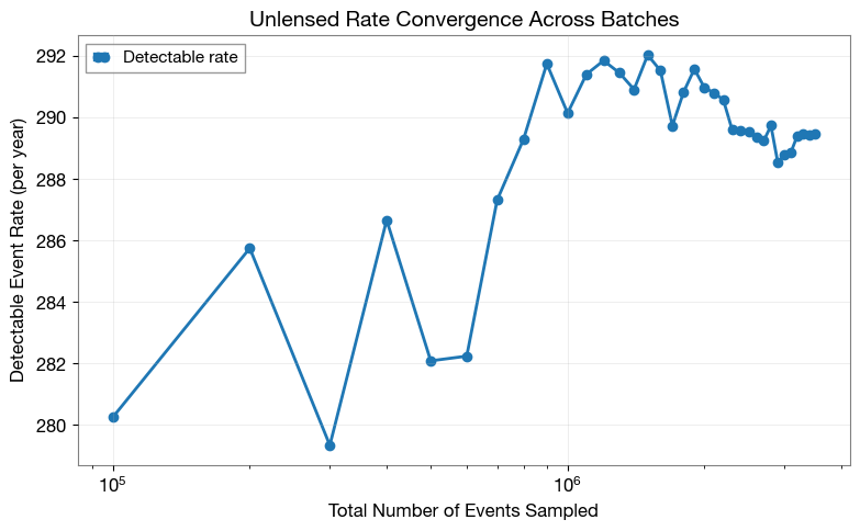
2.3 Rate Stability (Unlensed)
Quantify convergence using mean and standard deviation from the last few batches.
[7]:
import numpy as np

# Select rates from the last 4 batches
idx_converged = [-4, -3, -2, -1]
rates_converged = np.array(meta_data['total_rate'])[idx_converged]

if len(rates_converged) > 0:
    mean_rate = rates_converged.mean()
    std_rate = rates_converged.std()

    print(f"=== Unlensed Rate Stability Analysis ===")
    print(f"Number of batches analyzed: {len(rates_converged)}")
    print(f"Mean rate: {mean_rate:.4e} events/year")
    print(f"Standard deviation: {std_rate:.4e} events/year")
    print(f"Relative uncertainty: {(std_rate/mean_rate)*100:.3f}%")
else:
    print("Not enough batches to assess convergence.")

# Update the rate with the converged mean
detectable_rate_unlensed = mean_rate
=== Unlensed Rate Stability Analysis ===
Number of batches analyzed: 4
Mean rate: 3.5249e+02 events/year
Standard deviation: 1.8444e-01 events/year
Relative uncertainty: 0.052%
2.4 Lensed Events
Generate lensed detectable events. For lensed events, we can specify:
pdet_threshold: List of detection thresholds for each imagenum_img: Number of images that must meet each corresponding threshold
Here, stopping_criteria=None with size=1000 means sampling continues until at least 1000 detectable lensed events are collected.
[11]:
# Sample until we have at least 1,000 detectable lensed events
# use 'print(ler.selecting_n_lensed_detectable_events.__doc__)' to see all input args
# the choice of size, batch_size and stopping_criteria here is to run the test quickly. If you are comparing with the unlensed results, you should use the same size, batch_size and stopping_criteria as the unlensed case.
detectable_rate_lensed, lensed_param_detectable_n = ler.selecting_n_lensed_detectable_events(
    size=1000,                           # Target number of detectable events
    batch_size=50000,                    # Events per batch
    stopping_criteria=None,              # No stopping criteria (sample until size is reached)
    pdet_threshold=[0.5, 0.5],           # Detection thresholds for images
    num_img=[1, 1],                      # Number of images required per threshold
    resume=True,                        # Resume from previous state if available
    output_jsonfile='lensed_params_n_detectable.json',
    meta_data_file='meta_lensed.json',
    pdet_type='boolean',
    trim_to_size=False,
)

print(f"\n=== Lensed N-Event Sampling Results ===")
print(f"Detectable event rate: {detectable_rate_lensed:.4e} events per year")
print(f"Total detectable events collected: {len(lensed_param_detectable_n['zs'])}")
# initial batch will take longer as it needs to compile the numba njit functions; expected time: ~50s in first batch, then ~15s per subsequent batch
# time :
stopping criteria not set. sample collection will stop when number of detectable events exceeds the specified size.
Resuming from 141 detectable events.
collected number of detectable events =  141
collected number of detectable events (batch) =  66
collected number of detectable events (cumulative) =  207
total number of events =  150000
batch rate (yr^-1): 0.14672952652651622
total rate (yr^-1): 0.1533990504595397
collected number of detectable events (batch) =  66
collected number of detectable events (cumulative) =  273
total number of events =  200000
batch rate (yr^-1): 0.14672952652651622
total rate (yr^-1): 0.15173166947628383
collected number of detectable events (batch) =  72
collected number of detectable events (cumulative) =  345
total number of events =  250000
batch rate (yr^-1): 0.16006857439256314
total rate (yr^-1): 0.1533990504595397
collected number of detectable events (batch) =  66
collected number of detectable events (cumulative) =  411
total number of events =  300000
batch rate (yr^-1): 0.14672952652651622
total rate (yr^-1): 0.15228746313736913
collected number of detectable events (batch) =  53
collected number of detectable events (cumulative) =  464
total number of events =  350000
batch rate (yr^-1): 0.11782825615008122
total rate (yr^-1): 0.14736471928204226
collected number of detectable events (batch) =  67
collected number of detectable events (cumulative) =  531
total number of events =  400000
batch rate (yr^-1): 0.14895270117085738
total rate (yr^-1): 0.14756321701814415
collected number of detectable events (batch) =  75
collected number of detectable events (cumulative) =  606
total number of events =  450000
batch rate (yr^-1): 0.16673809832558661
total rate (yr^-1): 0.14969375938563775
collected number of detectable events (batch) =  57
collected number of detectable events (cumulative) =  663
total number of events =  500000
batch rate (yr^-1): 0.12672095472744582
total rate (yr^-1): 0.14739647891981855
collected number of detectable events (batch) =  46
collected number of detectable events (cumulative) =  709
total number of events =  550000
batch rate (yr^-1): 0.10226603363969312
total rate (yr^-1): 0.1432937111670799
collected number of detectable events (batch) =  67
collected number of detectable events (cumulative) =  776
total number of events =  600000
batch rate (yr^-1): 0.14895270117085738
total rate (yr^-1): 0.14376529366739468
collected number of detectable events (batch) =  82
collected number of detectable events (cumulative) =  858
total number of events =  650000
batch rate (yr^-1): 0.1823003208359747
total rate (yr^-1): 0.14672952652651622
collected number of detectable events (batch) =  72
collected number of detectable events (cumulative) =  930
total number of events =  700000
batch rate (yr^-1): 0.16006857439256314
total rate (yr^-1): 0.1476823156598053
collected number of detectable events (batch) =  76
collected number of detectable events (cumulative) =  1006
total number of events =  750000
batch rate (yr^-1): 0.16896127296992777
total rate (yr^-1): 0.14910091281381346
Given size=1000 reached

storing detectable lensed params in ./ler_data/lensed_params_n_detectable.json
storing meta data in ./ler_data/meta_lensed.json

=== Lensed N-Event Sampling Results ===
Detectable event rate: 1.4910e-01 events per year
Total detectable events collected: 1006
[12]:
# include other useful parameters in the output dictionary.
# It is omitted by default to save runtime and memory.
# For theta_E, n_images, mass_1, mass_2, luminosity_distance:
lensed_param_detectable_n = ler.recover_redundant_parameters(lensed_param_detectable_n)
# For effective_luminosity_distance, effective_geocent_time, effective_phase, effective_ra, effective_dec:
lensed_param_detectable_n = ler.produce_effective_params(lensed_param_detectable_n)

# or you can simply set 'include_redundant_parameters=True, include_effective_parameters=True' in the input args of LeR initialization to include these parameters in the output dictionary by default.
2.5 Rate Convergence (Lensed)
Visualize the lensed detection rate evolution across batches.
[13]:
import matplotlib.pyplot as plt
from ler.utils import get_param_from_json

# Load metadata containing rates for each batch
meta_data = get_param_from_json(ler.ler_directory + '/meta_lensed.json')

# Plot rate vs sampling size
plt.figure(figsize=(8, 5))
plt.plot(
    meta_data['events_total'],
    meta_data['total_rate'],
    'o-',
    linewidth=2,
    markersize=6,
    color='C1',
    label='Detectable rate'
)

plt.xlabel('Total Number of Events Sampled', fontsize=12)
plt.ylabel('Detectable Event Rate (per year)', fontsize=12)
plt.title('Lensed Rate Convergence Across Batches', fontsize=14, fontweight='bold')
plt.grid(alpha=0.3)
plt.legend(fontsize=11)
plt.xscale('log')
plt.tight_layout()
plt.show()
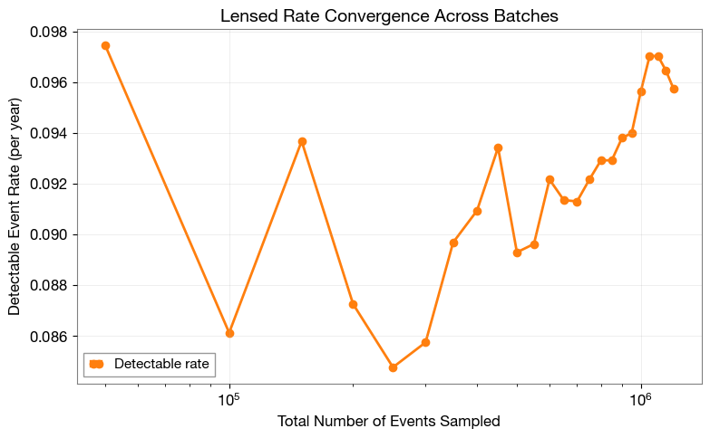
2.6 Rate Stability (Lensed)
Quantify convergence using mean and standard deviation from the last few batches.
[14]:
import numpy as np

# Select rates from the last 4 batches
idx_converged = [-4, -3, -2, -1]
rates_converged = np.array(meta_data['total_rate'])[idx_converged]

if len(rates_converged) > 0:
    mean_rate = rates_converged.mean()
    std_rate = rates_converged.std()

    print(f"=== Lensed Rate Stability Analysis ===")
    print(f"Number of batches analyzed: {len(rates_converged)}")
    print(f"Mean rate: {mean_rate:.4e} events/year")
    print(f"Standard deviation: {std_rate:.4e} events/year")
    print(f"Relative uncertainty: {(std_rate/mean_rate)*100:.3f}%")
else:
    print("Not enough batches to assess convergence.")

# Update the rate with the converged mean
detectable_rate_lensed = mean_rate
=== Lensed Rate Stability Analysis ===
Number of batches analyzed: 4
Mean rate: 1.4682e-01 events/year
Standard deviation: 1.9548e-03 events/year
Relative uncertainty: 1.331%
2.7 Rate Comparison
Compare detection rates between lensed and unlensed events.
[15]:
# Compare lensed vs unlensed rates
print(f"=== Detection Rate Comparison ===")
print(f"Unlensed detectable rate: {detectable_rate_unlensed:.4e} events/year")
print(f"Lensed detectable rate:   {detectable_rate_lensed:.4e} events/year")
print(f"Ratio (Unlensed/Lensed):  {(detectable_rate_unlensed/detectable_rate_lensed):.2f}")
=== Detection Rate Comparison ===
Unlensed detectable rate: 3.5249e+02 events/year
Lensed detectable rate:   1.4682e-01 events/year
Ratio (Unlensed/Lensed):  2400.85
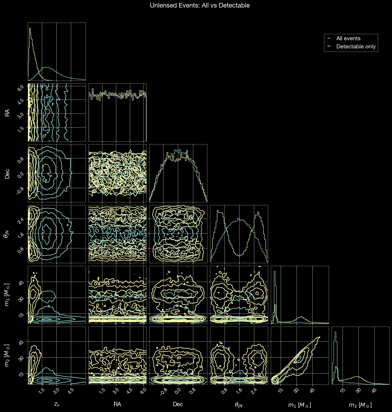
3. Parameter Distributions: All vs Detectable
Compare parameter distributions between all sampled events and detectable events. Corner plots reveal selection effects introduced by detector sensitivity.
3.1 Unlensed Events
Generate a large sample of all unlensed events (both detectable and non-detectable) for comparison.
[16]:
# Generate a large sample of all unlensed events for comparison
unlensed_param = ler.unlensed_cbc_statistics(size=50000, batch_size=50000, resume=True, output_jsonfile='unlensed_params_all.json')

print(f"Total unlensed events sampled: {len(unlensed_param['zs'])}")
unlensed params will be stored in ./ler_data/unlensed_params_all.json
removing ./ler_data/unlensed_params_all.json if it exists
resuming from ./ler_data/unlensed_params_all.json
Batch no. 1
sampling gw source params...
calculating pdet...
saving all unlensed parameters in ./ler_data/unlensed_params_all.json
Total unlensed events sampled: 50000
Corner plot comparing all sampled events vs detectable events:
[17]:
import corner
import numpy as np
import matplotlib.pyplot as plt
import matplotlib.lines as mlines
from ler.utils import get_param_from_json

# Load data
param = get_param_from_json('./ler_data/unlensed_params_all.json')
param_detectable = get_param_from_json('./ler_data/unlensed_params_n_detectable.json')

# select mass_1_source less than 90 solar masses to focus on the more common stellar-mass black hole events
mask_all = (param['mass_1_source'] < 60) & (param['zs'] < 6.0)
mask_detectable = (param_detectable['mass_1_source'] < 60) & (param_detectable['zs'] < 6.0)

# Parameters to compare
param_names = ['zs', 'ra', 'dec', 'theta_jn', 'mass_1_source', 'mass_2_source']
labels = ['$z_s$', 'RA', 'Dec', r'$\theta_{JN}$', '$m_1$ [$M_\odot$]', '$m_2$ [$M_\odot$]']

# Prepare data for corner plot
samples_all = np.stack([param[p][mask_all] for p in param_names], axis=1)
samples_detectable = np.stack([param_detectable[p][mask_detectable] for p in param_names], axis=1)

# Create corner plot for all events
fig = corner.corner(
    samples_all,
    labels=labels,
    color='C0',
    alpha=0.5,
    plot_density=False,
    plot_datapoints=False,
    smooth=0.8,
    bins=50,
    hist_kwargs={'density': True}
)

# Overlay detectable events
corner.corner(
    samples_detectable,
    labels=labels,
    color='C1',
    alpha=0.5,
    fig=fig,
    plot_density=False,
    plot_datapoints=False,
    smooth=0.8,
    bins=50,
    hist_kwargs={'density': True}
)

# Add legend
blue_line = mlines.Line2D([], [], color='C0', label='All events')
orange_line = mlines.Line2D([], [], color='C1', label='Detectable only')
fig.legend(handles=[blue_line, orange_line], loc='upper right',
           bbox_to_anchor=(0.95, 0.95), fontsize=14)
fig.suptitle('Unlensed Events: All vs Detectable', fontsize=16, y=1.02)

plt.show()
[18]:
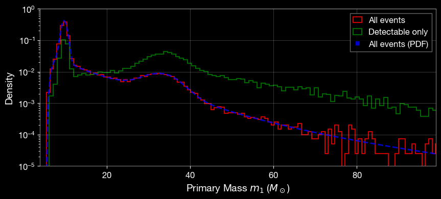
# plot param['mass_1_source']
plt.figure(figsize=(10, 4))
plt.hist(param['mass_1_source'], bins=300, alpha=0.8, linewidth=1.5, label='All events', density=True, histtype='step', color='r')
plt.hist(param_detectable['mass_1_source'], bins=300, alpha=0.8, linewidth=1.5, label='Detectable only', density=True, histtype='step', color='g')

mass_arr = np.linspace(4, 99, 200)
mass_pdf = ler.mass_1_source.pdf(mass_arr)
plt.plot(mass_arr, mass_pdf, 'b--', label='All events (PDF)', alpha=0.8, linewidth=2)

plt.xlabel('Primary Mass $m_1$ ($M_\\odot$)', fontsize=14)
plt.ylabel('Density', fontsize=14)
plt.yscale('log')
plt.ylim(1e-5, 1.0)
plt.xlim(4, 99)
plt.legend()
plt.grid(alpha=0.3)
plt.show()
3.2 Lensed Events
Compare intrinsic, strongly lensed, and detectable lensed event distributions. First, generate strongly lensed events:
[19]:
# Generate a large sample of all lensed events for comparison
lensed_param = ler.lensed_cbc_statistics(size=50000, batch_size=50000, resume=True, output_jsonfile='lensed_params_all.json')

print(f"Total lensed events sampled: {len(lensed_param['zs'])}")
lensed params will be stored in ./ler_data/lensed_params_all.json
removing ./ler_data/lensed_params_all.json if it exists
resuming from ./ler_data/lensed_params_all.json
Batch no. 1
sampling lensed params...
sampling lens parameters with epl_shear_sl_parameters_rvs...
computing image properties using ler's epl+shear (analytical, njit) solver...
Invalid sample found. Resampling 140 lensed events...
sampling lens parameters with epl_shear_sl_parameters_rvs...
computing image properties using ler's epl+shear (analytical, njit) solver...
calculating pdet...
saving all lensed parameters in ./ler_data/lensed_params_all.json
Total lensed events sampled: 50000
Generate intrinsic parameters (without strong lensing selection):
[20]:
# Generate a large sample of all lensed events for comparison
lensed_param_intrinsic = ler.sample_all_routine_epl_shear_intrinsic(size=50000)

print(f"Total lensed events sampled: {len(lensed_param_intrinsic['zs'])}")

# save to file
from ler.utils import append_json
append_json(ler.ler_directory+'/lensed_param_intrinsic.json', lensed_param_intrinsic, replace=True);
Total lensed events sampled: 50000
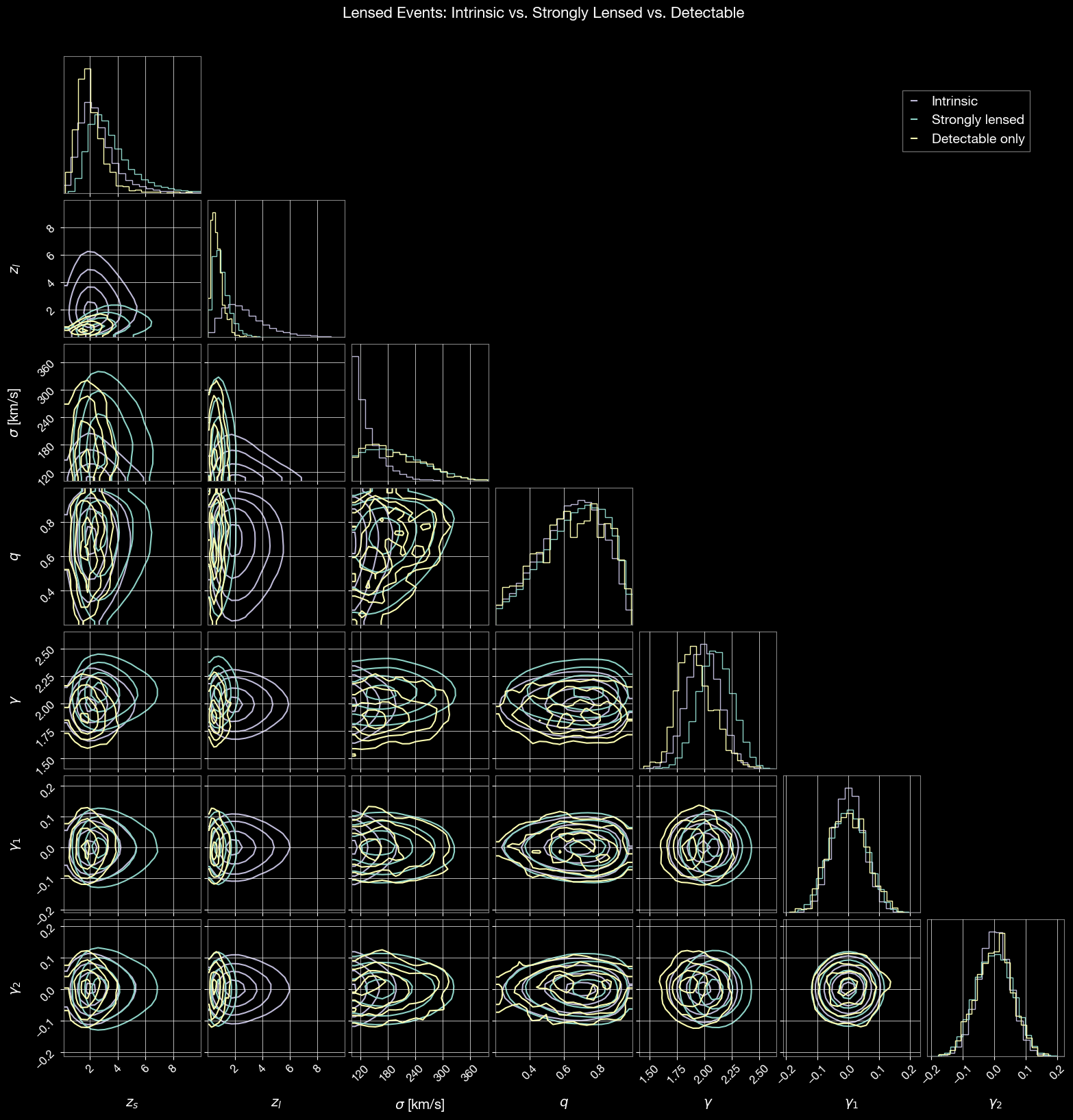
Corner plot comparing intrinsic, strongly lensed, and detectable events:
[21]:
import corner
import numpy as np
import matplotlib.pyplot as plt
import matplotlib.lines as mlines
from ler.utils import get_param_from_json
# Load data
param = get_param_from_json('./ler_data/lensed_params_all.json')
param_detectable = get_param_from_json('./ler_data/lensed_params_n_detectable.json')
param_intrinsic = get_param_from_json('./ler_data/lensed_param_intrinsic.json')
# lensed_param_intrinsic is already in memory from cell 24
# Lensing-specific parameters to compare
param_names = ['zs', 'zl', 'sigma', 'q', 'gamma', 'gamma1', 'gamma2']
labels = ['$z_s$', '$z_l$', r'$\sigma$ [km/s]', '$q$', r'$\gamma$', r'$\gamma_1$', r'$\gamma_2$']
# Prepare data for corner plot
samples_intrinsic = np.stack([param_intrinsic[p] for p in param_names], axis=1)
samples_all = np.stack([param[p] for p in param_names], axis=1)
samples_detectable = np.stack([param_detectable[p] for p in param_names], axis=1)
# Create corner plot for intrinsic events
fig = corner.corner(
samples_intrinsic,
labels=labels,
color='C2',
alpha=0.5,
plot_density=False,
plot_datapoints=False,
smooth=0.8,
hist_kwargs={'density': True}
)
# Overlay strongly lensed events
corner.corner(
samples_all,
labels=labels,
color='C0',
alpha=0.5,
fig=fig,
plot_density=False,
plot_datapoints=False,
smooth=0.8,
hist_kwargs={'density': True}
)
# Overlay detectable events
corner.corner(
samples_detectable,
labels=labels,
color='C1',
alpha=0.5,
fig=fig,
plot_density=False,
plot_datapoints=False,
smooth=0.8,
hist_kwargs={'density': True}
)
# Add legend
green_line = mlines.Line2D([], [], color='C2', label='Intrinsic')
blue_line = mlines.Line2D([], [], color='C0', label='Strongly lensed')
orange_line = mlines.Line2D([], [], color='C1', label='Detectable only')
fig.legend(handles=[green_line, blue_line, orange_line], loc='upper right',
bbox_to_anchor=(0.95, 0.95), fontsize=14)
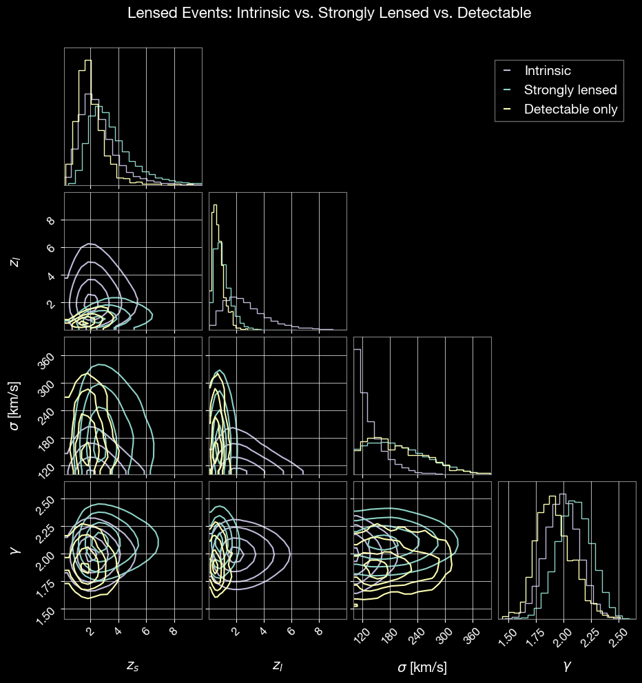
fig.suptitle('Lensed Events: Intrinsic vs. Strongly Lensed vs. Detectable', fontsize=16, y=1.02)
plt.show()
[22]:
import corner
import numpy as np
import matplotlib.pyplot as plt
import matplotlib.lines as mlines
from ler.utils import get_param_from_json

# Load data
param = get_param_from_json('./ler_data/lensed_params_all.json')
param_detectable = get_param_from_json('./ler_data/lensed_params_n_detectable.json')
param_intrinsic = get_param_from_json('./ler_data/lensed_param_intrinsic.json')
# lensed_param_intrinsic is already in memory from cell 24

# Lensing-specific parameters to compare
param_names = ['zs', 'zl', 'sigma', 'gamma']
labels = ['$z_s$', '$z_l$', r'$\sigma$ [km/s]', r'$\gamma$']

# Prepare data for corner plot
samples_intrinsic = np.stack([param_intrinsic[p] for p in param_names], axis=1)
samples_all = np.stack([param[p] for p in param_names], axis=1)
samples_detectable = np.stack([param_detectable[p] for p in param_names], axis=1)

# Create corner plot for intrinsic events
fig = corner.corner(
    samples_intrinsic,
    labels=labels,
    color='C2',
    alpha=0.5,
    plot_density=False,
    plot_datapoints=False,
    smooth=0.8,
    hist_kwargs={'density': True}
)

# Overlay strongly lensed events
corner.corner(
    samples_all,
    labels=labels,
    color='C0',
    alpha=0.5,
    fig=fig,
    plot_density=False,
    plot_datapoints=False,
    smooth=0.8,
    hist_kwargs={'density': True}
)

# Overlay detectable events
corner.corner(
    samples_detectable,
    labels=labels,
    color='C1',
    alpha=0.5,
    fig=fig,
    plot_density=False,
    plot_datapoints=False,
    smooth=0.8,
    hist_kwargs={'density': True}
)

# Add legend
green_line = mlines.Line2D([], [], color='C2', label='Intrinsic')
blue_line = mlines.Line2D([], [], color='C0', label='Strongly lensed')
orange_line = mlines.Line2D([], [], color='C1', label='Detectable only')
fig.legend(handles=[green_line, blue_line, orange_line], loc='upper right',
           bbox_to_anchor=(0.95, 0.95), fontsize=14)
fig.suptitle('Lensed Events: Intrinsic vs. Strongly Lensed vs. Detectable', fontsize=16, y=1.02)

plt.show()
4. Visualizing Lensed Detectable Events
Visualize properties of detectable lensed events. An example event is highlighted in each plot to show individual characteristics within the population.
4.1 Redshift Distribution
Compare redshift distributions of intrinsic and detected populations.
[23]:
from ler.utils import get_param_from_json
import numpy as np
import matplotlib.pyplot as plt
from matplotlib.ticker import AutoMinorLocator

np.random.seed(100)

# Load data
unlensed_params_det = get_param_from_json('./ler_data/unlensed_params_n_detectable.json')
lensed_params_det = get_param_from_json('./ler_data/lensed_params_n_detectable.json')
unlensed_params = get_param_from_json('./ler_data/unlensed_params_all.json')
lensed_params = get_param_from_json('./ler_data/lensed_params_all.json')
lensed_params_intrinsic = get_param_from_json('./ler_data/lensed_param_intrinsic.json')

bbh_pop_intrinsic = unlensed_params['zs']
unlensed_bbh_pop_detected = unlensed_params_det['zs']
lensed_bbh_pop_detected = lensed_params_det['zs']
lens_detected = lensed_params_det['zl']
lens_dist_intrinsic = lensed_params_intrinsic['zl']

# create gaussian kde
from scipy.stats import gaussian_kde
bandwidth = 0.4
kde_bbh_pop_intrinsic = gaussian_kde(bbh_pop_intrinsic, bw_method=bandwidth)
kde_unlensed_bbh_pop_detected = gaussian_kde(unlensed_bbh_pop_detected, bw_method=bandwidth)
kde_lensed_bbh_pop_detected = gaussian_kde(lensed_bbh_pop_detected, bw_method=bandwidth)
kde_lens_dist_intrinsic = gaussian_kde(lens_dist_intrinsic, bw_method=bandwidth)
kde_lens_detected = gaussian_kde(lens_detected, bw_method=bandwidth)

# Choose a random detected lensed event to highlight
pdet = lensed_params_det['pdet_net']
idx_4img = pdet > 0.5
idx_4img = np.sum(idx_4img, axis=1) ==2 # 2 images detected
chosen_idx_list = np.where(idx_4img)[0]
chosen_idx = chosen_idx_list[10]  # pick the 10th one for consistency
print(f"Chosen detected lensed event index: {chosen_idx}")

# ---------- Data ----------
z = np.linspace(0, 5, 1000)

# ---------- Plot ----------
fig, ax = plt.subplots(figsize=(8, 4))

colors = {
    "black": "#000000",
    "violet": "#7E57C2",
    "brown": "#8D6E63",
    "grey": "#616161",
    "red": "#E53935",
    "blue": "#1E88E5",
}

# intrinsic distributions
ax.plot(z, kde_bbh_pop_intrinsic(z), label='Intrinsic BBH population',
        color=colors["grey"], linestyle='--', linewidth=1.2)
ax.plot(z, kde_lens_dist_intrinsic(z), label='Intrinsic Lens population',
        color=colors["brown"], linestyle='--', linewidth=1.2)

# detected distributions
ax.plot(z, kde_unlensed_bbh_pop_detected(z), label='Detected Unlensed BBH population',
        color=colors["black"], linestyle='-', linewidth=1.4)
ax.plot(z, kde_lensed_bbh_pop_detected(z), label='Detected Lensed BBH population',
        color=colors["red"], linestyle='-', linewidth=1.4)
ax.plot(z, kde_lens_detected(z), label='Lenses associated with detectable events',
        color=colors["violet"], linestyle='-', linewidth=1.4)

# Example detected lensed event redshifts
ax.axvline(lensed_params_det['zs'][chosen_idx],
           color=colors["red"], linestyle=':', linewidth=2,
           label='Example detected lensed event source redshift')
ax.axvline(lensed_params_det['zl'][chosen_idx],
           color=colors["brown"], linestyle=':', linewidth=2,
           label='Example detected lensed event lens redshift')

# ---------- Legend ----------
legend = ax.legend(
    handlelength=2.0,
    loc='upper right',
    bbox_to_anchor=(1, 1),
    frameon=True,
    fontsize=10.,
    edgecolor='lightgray'
)
legend.get_frame().set_boxstyle('Round', pad=0.0, rounding_size=0.2)
for handle in legend.get_lines():
    handle.set_linewidth(1.5)
    handle.set_alpha(0.8)

# ---------- Axes labels, limits, and grid ----------
ax.set_xlabel(r'Redshift $z$', fontsize=11)
ax.set_ylabel(r'Probability Density', fontsize=11)
ax.set_xlim(0, 5)
ax.set_ylim(0, None)

ax.grid(alpha=0.4, linestyle='--', linewidth=0.5)
ax.xaxis.set_minor_locator(AutoMinorLocator())
ax.yaxis.set_minor_locator(AutoMinorLocator())

# add title
ax.set_title('Redshift Distributions of BBH and Lens Populations', fontsize=12)

plt.tight_layout()
# plt.savefig('lens_paramters_baseline_redshift_distributions.svg',
#             dpi=300, bbox_inches='tight', transparent=True)
plt.show()
Chosen detected lensed event index: 13
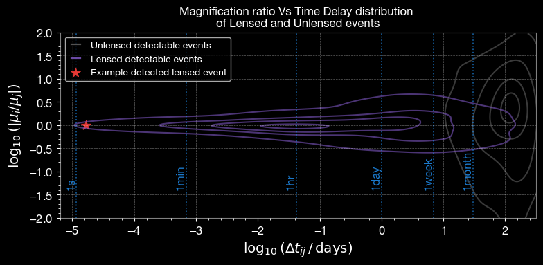
4.2 Magnification Ratio vs Time Delay
Relative magnification vs time delay distinguishes lensed from unlensed events.
[24]:
from ler.utils import relative_mu_dt_unlensed, relative_mu_dt_lensed, mu_vs_dt_plot

# for unlensed detectable events
dmu_unlensed, dt_unlensed = relative_mu_dt_unlensed(param=unlensed_params_det)

# for lensed detectable events
lensed_dict = relative_mu_dt_lensed(lensed_param=lensed_params_det)
dt_lensed = np.concatenate((lensed_dict['dt_rel0'], lensed_dict['dt_rel90']))
dmu_lensed = np.concatenate((lensed_dict['mu_rel0'], lensed_dict['mu_rel90']))

# chosen example index for 4 images, find time delays and magnifications
chosen_lens_dt = lensed_params_det['time_delays'][chosen_idx]
chosen_lens_mu = lensed_params_det['magnifications'][chosen_idx]
pdet = lensed_params_det['pdet_net'][chosen_idx]

dt_lensed_chosen = np.log10((chosen_lens_dt[2]-chosen_lens_dt[1])/ (60 * 60 * 24))
dmu_lensed_chosen = np.log10(abs(chosen_lens_mu[2]/chosen_lens_mu[1]))

# ---------------------------------------
# Plot Magnification ratio Vs Time Delay
# ---------------------------------------
fig, ax = plt.subplots(figsize=(8, 4))

colors = {
    "black": "#000000",
    "violet": "#7E57C2",
    "brown": "#8D6E63",
    "grey": "#616161",
    "red": "#E53935",
    "blue": "#1E88E5",
}

# Use your existing helper without modification
mu_vs_dt_plot(dt_unlensed, dmu_unlensed, colors=[colors['grey']]*5)
mu_vs_dt_plot(dt_lensed,   dmu_lensed,   colors=[colors['violet']]*5)

# Proxy artists for legend
# Proxy artists for legend
ax.plot([], [], color=colors['grey'],  linestyle='-', label='Unlensed detectable events', linewidth=1.5)
ax.plot([], [], color=colors['violet'], linestyle='-', label='Lensed detectable events',   linewidth=1.5)

# Chosen example point
ax.scatter(
    dt_lensed_chosen, dmu_lensed_chosen,
    color=colors['red'], marker='*', s=110, linewidths=0.6,
    label='Example detected lensed event'
)

# plot line for 1s, 1hr, 1day, 1week, 1month time delays
time_delays = [1, 60, 60*60, 60*60*24, 60*60*24*7, 60*60*24*30]
labels_td = ['1s', '1min', '1hr', '1day', '1week', '1month']
for td in time_delays:
    ax.axvline(np.log10(td/(60*60*24)), color=colors['blue'], linestyle=':', linewidth=1.2, alpha=0.7)
    ax.text(np.log10(td/(60*60*24)), ax.get_ylim()[1]*-0.7, labels_td[time_delays.index(td)], color=colors['blue'], fontsize=12, rotation=90, va='bottom', ha='right', alpha=0.9)

# ---------- Legend ----------
legend = ax.legend(
    handlelength=1.5,
    loc='upper left',
    bbox_to_anchor=(0, 1),
    frameon=True,
    fontsize=10,
    edgecolor='lightgray'
)
legend.get_frame().set_boxstyle('Round', pad=0.0, rounding_size=0.2)
for handle in legend.get_lines():
    handle.set_linewidth(1.6)
    handle.set_alpha(0.85)

# add title
ax.set_title('Magnification ratio Vs Time Delay distribution \nof Lensed and Unlensed events', fontsize=12)

# ---------- Axes, ticks, grid ----------
ax.set_xlabel(r'$\log_{10}(\Delta t_{ij} \,/\, \mathrm{days})$')
ax.set_ylabel(r'$\log_{10}(|\mu_i / \mu_j|)$')
ax.set_xlim(-5.2, 2.5)
ax.set_ylim(-2, 2)

ax.xaxis.set_minor_locator(AutoMinorLocator())
ax.yaxis.set_minor_locator(AutoMinorLocator())
ax.grid(alpha=0.38, linestyle='--', linewidth=0.5)

plt.tight_layout()
# plt.savefig('mu_vs_dt_science_ieee.svg', dpi=600, bbox_inches='tight', transparent=True)
plt.show()
# time: 32s
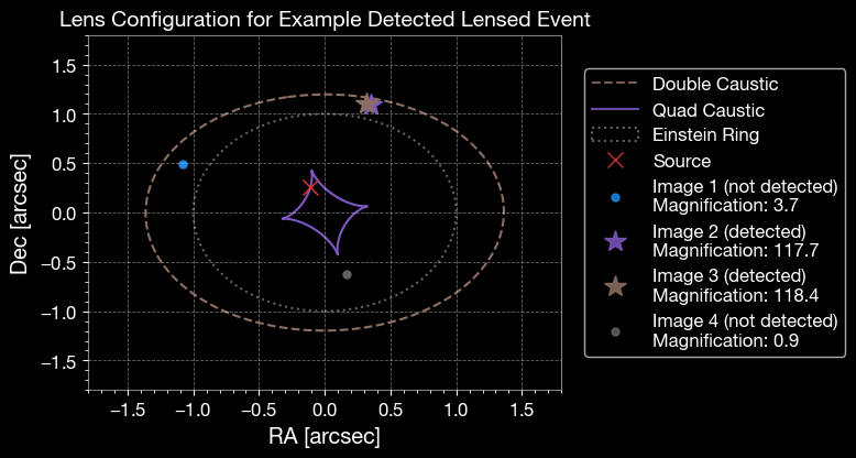
4.3 Caustic Plot
Lens configuration for an example event, showing caustics, critical curves, and image positions.
[25]:
# include other useful parameters in the output dictionary.
# It is omitted by default to save runtime and memory.
# For theta_E, n_images, mass_1, mass_2, luminosity_distance:
lensed_params_det = ler.recover_redundant_parameters(lensed_params_det)
[26]:
from ler.image_properties.cross_section_njit import caustic_points_epl_shear
from ler.image_properties.epl_shear_njit import image_position_analytical_njit

# ---------- Custom color palette ----------
colors = {
    "black": "#000000",
    "violet": "#7E57C2",
    "brown":  "#8D6E63",
    "grey":   "#616161",
    "red":    "#E53935",
    "blue":   "#1E88E5",
    "green":  "#43A047",
    "orange": "#FB8C00",
}

# ----- Lens parameters -----
q   = lensed_params_det['q'][chosen_idx]
phi = lensed_params_det['phi'][chosen_idx]
gamma = lensed_params_det['gamma'][chosen_idx]
gamma1 = lensed_params_det['gamma1'][chosen_idx]
gamma2 = lensed_params_det['gamma2'][chosen_idx]
theta_E = lensed_params_det['theta_E'][chosen_idx]

# ----- Solve image configuration -----
# unscaled source position
beta_ra  = lensed_params_det['x_source'][chosen_idx] / theta_E
beta_dec = lensed_params_det['y_source'][chosen_idx] / theta_E

x_img, y_img, fermat_pot, mu, image_type, nimg = image_position_analytical_njit(
    beta_ra, beta_dec, q, phi, gamma, gamma1, gamma2,
    theta_E=1.0, magnification_limit=1.0/100.0,
)
theta_ra = x_img[:nimg]
theta_dec = y_img[:nimg]
magnifications = np.abs(mu[:nimg])

# ----- Figure -----
fig, ax = plt.subplots(figsize=(8, 7))  # wider figure

# Caustics
cp = caustic_points_epl_shear(1.0, q, phi, gamma, gamma1, gamma2, num_th=500, maginf=-100.0, quad=False)
ax.plot(cp[0], cp[1], color=colors['brown'], linewidth=1.5, linestyle='--', label='Double Caustic')
cp = caustic_points_epl_shear(1.0, q, phi, gamma, gamma1, gamma2, num_th=500, maginf=-100.0, quad=True)
ax.plot(cp[0], cp[1], color=colors['violet'], linewidth=1.5, linestyle='-', label='Quad Caustic')

# Einstein ring
circle = plt.Circle((0, 0), 1.0, color=colors['grey'], fill=False,
                    linestyle='dotted', linewidth=1.5, label='Einstein Ring')
ax.add_artist(circle)

# Source position
ax.plot(beta_ra, beta_dec, marker='x', ls='None', color=colors['red'], label='Source', markersize=10)

# Image positions
img_colors = [colors['blue'], colors['violet'], colors['brown'], colors['grey']]
pdet_image = lensed_params_det['pdet_net'][chosen_idx]
for i in range(nimg):
    if pdet_image[i] >= 0.5:
        ax.plot(theta_ra[i], theta_dec[i], marker='*', ls='None',
                color=img_colors[i % len(img_colors)],
                label=f'Image {i+1} (detected)\nMagnification: {magnifications[i]:.1f}', markersize=15)
    else:
        ax.plot(theta_ra[i], theta_dec[i], marker='.', ls='None',
                color=img_colors[i % len(img_colors)],
                label=f'Image {i+1} (not detected)\nMagnification: {magnifications[i]:.1f}', markersize=10)
# Axes & Grid
ax.set_xlabel('RA [arcsec]')
ax.set_ylabel('Dec [arcsec]')
dim_x, dim_y = 1.8, 1.8  # rectangular window
ax.set_xlim(-dim_x, dim_x)
ax.set_ylim(-dim_y, dim_y)

# Relax the aspect ratio → visually rectangular (with adjustable='box' to respect figure size)
ax.set_aspect(6/8, adjustable='box')

ax.xaxis.set_minor_locator(AutoMinorLocator())
ax.yaxis.set_minor_locator(AutoMinorLocator())
ax.grid(alpha=0.4, linestyle='--', linewidth=0.6)

# Legend on the side
legend = ax.legend(
    handlelength=2.5,
    loc='center left',
    bbox_to_anchor=(1.03, 0.5),
    frameon=True,
    fontsize=12,
    edgecolor='lightgray',
    numpoints=1,  # Show only one marker per legend entry
    scatterpoints=1
)
legend.get_frame().set_boxstyle('Round', pad=0.0, rounding_size=0.2)
for handle in legend.get_lines():
    handle.set_linewidth(1.5)
    handle.set_alpha(0.85)
# add title
ax.set_title('Lens Configuration for Example Detected Lensed Event', fontsize=14)
plt.tight_layout()
# plt.savefig('lens_configuration_rectangular.svg', dpi=600, bbox_inches='tight', transparent=True)
plt.show()
If you want to use lenstronomy to solve the lens configuration and plot the lensing caustics, critical curves, and image positions, you can use the following code snippet:
[ ]:
# from lenstronomy.LensModel.lens_model import LensModel
# from lenstronomy.LensModel.Solver.lens_equation_solver import LensEquationSolver
# from lenstronomy.LensModel.Solver.epl_shear_solver import caustics_epl_shear
# # import phi_q2_ellipticity
# from lenstronomy.Util.param_util import phi_q2_ellipticity

# # ---------- Custom color palette ----------
# colors = {
#     "black": "#000000",
#     "violet": "#7E57C2",
#     "brown":  "#8D6E63",
#     "grey":   "#616161",
#     "red":    "#E53935",
#     "blue":   "#1E88E5",
#     "green":  "#43A047",
#     "orange": "#FB8C00",
# }

# # ----- Lens setup -----
# lens_model_list = ["EPL", "SHEAR"]
# lensModel = LensModel(lens_model_list=lens_model_list)
# lens_eq_solver = LensEquationSolver(lensModel)

# q   = lensed_params_det['q'][chosen_idx]
# phi = lensed_params_det['phi'][chosen_idx]
# e1, e2 = phi_q2_ellipticity(phi, q)
# kwargs_spep = {
#     'theta_E': 1.0,
#     'e1': e1,
#     'e2': e2,
#     'gamma': lensed_params_det['gamma'][chosen_idx],
#     'center_x': 0.0,
#     'center_y': 0.0,
# }
# kwargs_shear = {
#     'gamma1': lensed_params_det['gamma1'][chosen_idx],
#     'gamma2': lensed_params_det['gamma2'][chosen_idx]
# }
# kwargs_lens = [kwargs_spep, kwargs_shear]

# # ----- Solve image configuration -----
# theta_E = lensed_params_det['theta_E'][chosen_idx]
# # unscaled source position
# beta_ra  = lensed_params_det['x_source'][chosen_idx]/theta_E
# beta_dec = lensed_params_det['y_source'][chosen_idx]/theta_E
# theta_ra, theta_dec = lens_eq_solver.image_position_from_source(
#     sourcePos_x=beta_ra, sourcePos_y=beta_dec, kwargs_lens=kwargs_lens,
#     solver="analytical", magnification_limit=1.0/100.0, arrival_time_sort=True
# )
# magnifications = lensModel.magnification(theta_ra, theta_dec, kwargs_lens)
# magnifications = np.abs(np.array(magnifications))
# # print(f"Magnifications calculated: {magnifications}")

# # ----- Figure -----
# fig, ax = plt.subplots(figsize=(8, 7))  # wider figure

# # Caustics
# cp = caustics_epl_shear(kwargs_lens, return_which="double", maginf=-100)
# ax.plot(cp[0], cp[1], color=colors['brown'], linewidth=1.5, linestyle='--', label='Double Caustic')
# cp = caustics_epl_shear(kwargs_lens, return_which="quad", maginf=-100)
# ax.plot(cp[0], cp[1], color=colors['violet'], linewidth=1.5, linestyle='-', label='Quad Caustic')

# # Einstein ring
# theta_E = 1.0
# circle = plt.Circle((0, 0), theta_E, color=colors['grey'], fill=False,
#                     linestyle='dotted', linewidth=1.5, label='Einstein Ring')
# ax.add_artist(circle)

# # Source position
# ax.plot(beta_ra, beta_dec, marker='x', ls='None', color=colors['red'], label='Source', markersize=10)

# # Image positions
# img_colors = [colors['blue'], colors['violet'], colors['brown'], colors['black']]
# pdet_image = lensed_params_det['pdet_net'][chosen_idx]
# for i in range(len(theta_ra)):
#     if pdet_image[i] >= 0.5:
#         ax.plot(theta_ra[i], theta_dec[i], marker='*', ls='None',
#                 color=img_colors[i % len(img_colors)],
#                 label=f'Image {i+1} (detected)\nMagnification: {magnifications[i]:.1f}', markersize=15)
#     else:
#         ax.plot(theta_ra[i], theta_dec[i], marker='.', ls='None',
#                 color=img_colors[i % len(img_colors)],
#                 label=f'Image {i+1} (not detected)\nMagnification: {magnifications[i]:.1f}', markersize=10)
# # Axes & Grid
# ax.set_xlabel('RA [arcsec]')
# ax.set_ylabel('Dec [arcsec]')
# dim_x, dim_y = 1.8, 1.8  # rectangular window
# ax.set_xlim(-dim_x, dim_x)
# ax.set_ylim(-dim_y, dim_y)

# # Relax the aspect ratio → visually rectangular (with adjustable='box' to respect figure size)
# ax.set_aspect(6/8, adjustable='box')

# ax.xaxis.set_minor_locator(AutoMinorLocator())
# ax.yaxis.set_minor_locator(AutoMinorLocator())
# ax.grid(alpha=0.4, linestyle='--', linewidth=0.6)

# # Legend on the side
# legend = ax.legend(
#     handlelength=2.5,
#     loc='center left',
#     bbox_to_anchor=(1.03, 0.5),
#     frameon=True,
#     fontsize=12,
#     edgecolor='lightgray',
#     numpoints=1,  # Show only one marker per legend entry
#     scatterpoints=1
# )
# legend.get_frame().set_boxstyle('Round', pad=0.0, rounding_size=0.2)
# for handle in legend.get_lines():
#     handle.set_linewidth(1.5)
#     handle.set_alpha(0.85)
# # add title
# ax.set_title('Lens Configuration for Example Detected Lensed Event', fontsize=14)
# plt.tight_layout()
# # plt.savefig('lens_configuration_rectangular.svg', dpi=600, bbox_inches='tight', transparent=True)
# plt.show()
5. Summary
This notebook demonstrated advanced sampling capabilities of LeR for generating detectable GW events.
Key Takeaways:
N-Event Sampling:
selecting_n_unlensed_detectable_eventsandselecting_n_lensed_detectable_eventscollect a target number of detectable events with convergence monitoring.Rate Convergence: Tracking rates across batches verifies statistical stability.
Resume Capability: Sampling can be interrupted and resumed without losing progress.
Selection Effects: The corner plots reveal how detector sensitivity and strong lensing selection bias the observed populations:
Detector sensitivity effects:
Lower redshift events are preferentially detected
Higher mass events have higher detection probability
Sky location and orientation effects are visible
Strong lensing selection effects:
Higher magnification events are more likely to be detected
Lensed events tend to occur at higher redshifts
Lens velocity dispersion influences strong lensing due to increased lensing cross-section
Lens galaxy density profile slope affects detectability
Lensing Visualization: The redshift distributions, magnification-time delay plots, and caustic diagrams provide insight into the properties of detectable lensed events.