Analytical Formulation for Gravitational Wave Event Rates

Written by Phurailatpam Hemantakumar. Last updated: 2026-02-06.

Overview

This document presents the analytical framework for calculating gravitational-wave (GW) event rates from compact-binary coalescences (CBCs), encompassing binary black holes (BBH), binary neutron stars (BNS), and neutron star–black hole binaries (NSBH). The formulation integrates cosmic merger rate densities with detector sensitivity functions to predict annual detection rates. Implementation examples using the ler package demonstrate practical applications of this framework.

Table of Contents

• Introduction

• Parameter-Marginalized Event Rate

• Redshift Distribution and Intrinsic Merger Rates

• Detection Criterion and SNR Modeling

• Complete Expression for GW (unlensed) Event Rate

• Simulation Results

  • Simulation Settings

  • GW Source Parameter Priors

  • Plot Comparison for Detectable and Intrinsic Populations

  • Rate Estimates for Different GW Detector Networks

Introduction

The annual rate of detectable (unlensed) GW events, \(\frac{\Delta N^{\rm obs}_{\rm U}}{\Delta t}\), gives the expected number of observed CBC mergers per year for a given detector network. It is obtained by combining the total intrinsic merger rate in the detector-frame, \(\frac{\Delta N_{\rm U}}{\Delta t}\), with the population-averaged probability of detection, \(P({\rm obs})\), such that

\[ \begin{split} \frac{\Delta N^{\rm obs}_{\rm U}}{\Delta t} = \frac{\Delta N_{\rm U}}{\Delta t} \times P({\rm obs}) \,. \end{split} \]

Parameter-Marginalized Event Rate

The observed event rate is obtained by averaging the detection probability over the GW parameters that determine the emitted signal and its projection onto a detector network. Given a joint prior \(P(\vec{\theta})\) and a conditional detection probability \(P({\rm obs}\mid\vec{\theta})\), the population-averaged detection probability is

\[ \begin{split} P({\rm obs}) = \int P({\rm obs}\mid \vec{\theta})\,P(\vec{\theta})\,d\vec{\theta} \,, \end{split} \]

so the annual detectable rate becomes

\[ \begin{split} \frac{\Delta N^{\rm obs}_{\rm U}}{\Delta t} = \frac{\Delta N_{\rm U}}{\Delta t} \int P({\rm obs} \mid \vec{\theta})\, P(\vec{\theta})\, d\vec{\theta} \,. \end{split} \]

Here \(\vec{\theta}\) denotes the full parameter set specifying the source and its configuration relative to the observer. It is convenient to write \(\vec{\theta}=\{\vec{\theta}_{\rm int},\vec{\theta}_{\rm ext}\}\), where the intrinsic parameters \(\vec{\theta}_{\rm int}\) describe the binary’s source-frame properties and the extrinsic parameters \(\vec{\theta}_{\rm ext}\) describe the source location and orientation in a geocentric equatorial frame that is independent of any particular detector. In this work,

\[ \begin{split} \vec{\theta}_{\rm int} = \{m^{\rm src}_1, m^{\rm src}_2, a_1, a_2, \theta_1, \theta_2, \phi_{12}, \phi_{\rm JL}\} \,, \end{split} \]

and

\[ \begin{split} \vec{\theta}_{\rm ext} = \{z_s, \iota, \phi, \psi, {\rm RA}, {\rm Dec}, t_c\} \, . \end{split} \]

The sampling priors and parameter ranges are summarized in Table 1, with visual references in Figure 1 and Figure 2. The ler package samples source distance through the redshift \(z_s\) rather than the luminosity distance \(d_L\), and it samples source-frame component masses \(m^{\rm src}_{1,2}\) rather than the redshifted detector-frame masses \(m_{1,2}=(1+z_s)m^{\rm src}_{1,2}\). Evaluating \(P({\rm obs}\mid\vec{\theta})\) therefore requires an internal mapping to the detector-frame parameterization used by waveform and SNR calculations. In ler, the conversion \(z_s\mapsto d_L\) is performed using the assumed cosmology and the mass redshifting \(m^{\rm src}_{1,2}\mapsto m_{1,2}\) is applied internally, while the projection from the geocentric sky frame to each interferometer is handled by the gwsnr backend following the conventions of bilby and LALSimulation.

Figure 1: Interactive visualization of the gravitational-wave coordinate system following the LALSimulation conventions. The figure shows three frames: the Equatorial (Observer) frame (blue), the Wave frame (green), and the Source (Orbital) frame (yellow). In the equatorial frame, the \(z\) axis is aligned with Earth’s rotation axis and the \(x\) axis points toward the vernal equinox; the sky position is specified by \(({\rm RA},{\rm Dec})\), with \({\rm RA}\) measured in the equatorial plane from the vernal equinox and \({\rm Dec}\) measured from the equatorial plane toward the north celestial pole. In the wave frame, the \(z\) axis is along the GW propagation direction toward the geocentre and the \((x,y)\) axes span the wave plane, with the wave-frame \(x\) axis defining the polarization basis. In the source frame, the \(z\) axis is aligned with the orbital angular momentum and the \((x,y)\) axes lie in the orbital plane; the inclination \(\iota\) is the angle between the line of sight and the orbital angular momentum (defined at \(f_{\rm ref}\) for precessing systems). The polarization angle \(\psi\) is measured in the wave plane from the ascending line of nodes, defined by the intersection of the equatorial plane with the wave plane, to the wave-frame \(x\) axis, with rotation about the wave-frame \(z\) axis; see the LALSimulation polarization convention for details Ref. The ring of test points in the wave plane illustrates the action of the \(h_{+,\times}\) polarizations on the observed strain, wrt the wave-frame axes. The sizes and distances in the figure are not to scale, and the visualization is meant for qualitative understanding of the coordinate systems and angles rather than a quantitative representation of any particular system.

Figure 2: Interactive spin-orientation visualization for a precessing BBH system. The figure shows the total angular momentum \(\mathbf{J}\) (purple) and the orbital angular momentum \(\mathbf{L}\) (green), together with the component spin vectors (red and blue) labelled by their dimensionless magnitudes \(a_1\) and \(a_2\). The tilt angles \(\theta_1\) and \(\theta_2\) are defined relative to \(\mathbf{L}\), and \(\phi_{12}\) is the azimuthal separation between the two spin vectors about \(\mathbf{L}\). The angle \(\phi_{\rm JL}\) parameterizes the azimuthal location of \(\mathbf{L}\) around \(\mathbf{J}\) at the chosen reference frequency \(f_{\rm ref}\); equivalently, this is the angle between the projections of \(\mathbf{L}\) and the line of sight onto the plane orthogonal to \(\mathbf{J}\) at \(f_{\rm ref}\). The precession of the orbital plane is illustrated by the motion of \(\mathbf{L}\) around \(\mathbf{J}\). The length of the vectors is not to scale, and the figure is meant for qualitative visualization of the spin angles rather than a quantitative representation of the system’s angular momenta.

Redshift Distribution and Intrinsic Merger Rates

The ler package uses redshift \(z_s\) to represent source distance rather than luminosity distance \(D_L\), and assumes that \(z_s\) is uncorrelated with the other source parameters. The redshift probability density \(P(z_s)\) is defined as the normalized distribution of sources over cosmic history and is proportional to the detector-frame intrinsic merger rate density \(\frac{d^2 N}{dt \, dV_c}\) and the comoving volume element \(\frac{dV_c}{dz_s}\). Equivalently, using the source-frame intrinsic merger rate density \(\frac{d^2 N}{d\tau dV_c}\) (or \(R_{\rm U}(z_s)\)), it can be written as

\[\begin{split} \begin{split} P(z_s) & \propto \frac{d^2 N}{dt \, dV_c} \frac{dV_c}{dz_s} \\ &\propto \frac{d^2 N}{d\tau \, dV_c} \frac{d\tau}{dt} \frac{dV_c}{dz_s} \\ &\propto \frac{R_{\rm U}(z_s)}{(1+z_s)} \frac{dV_c}{dz_s} \,, \end{split} \end{split}\]

where \(R_{\rm U}(z_s)\) is expressed per unit source-frame proper time \(\tau\) and per unit comoving volume, with \(\frac{d\tau}{dt} = \frac{1}{1+z_s}\). The factor \(\frac{1}{1+z_s}\) accounts for cosmological time dilation between the source-frame time \(\tau\) and the detector-frame time \(t\) (Dominik et al. 2013). The term \(\frac{dV_c}{dz_s}dz_s\) represents the comoving shell volume element at redshift \(z_s\), and the integration over \(z_s\) in the event-rate calculation is carried out over the full redshift range of interest.

Normalizing the redshift distribution introduces the constant \({\cal N}_{\rm U}\), which is equal to the total intrinsic merger rate per year in the detector-frame. The normalized form becomes

\[ \begin{split} P(z_s) = \frac{1}{{\cal N}_{\rm U}} \frac{R_{\rm U}(z_s)}{1+z_s} \frac{dV_c}{dz_s} \,, \end{split} \]

with

\[ \begin{split} {\cal N}_{\rm U} = \int_{z_{\rm min}}^{z_{\rm max}} \frac{R_{\rm U}(z_s)}{1+z_s} \frac{dV_c}{dz_s} \, dz_s \,. \end{split} \]

For visualization, \(R_{\rm U}(z_s)\) and \(P(z_s)\) are plotted below.

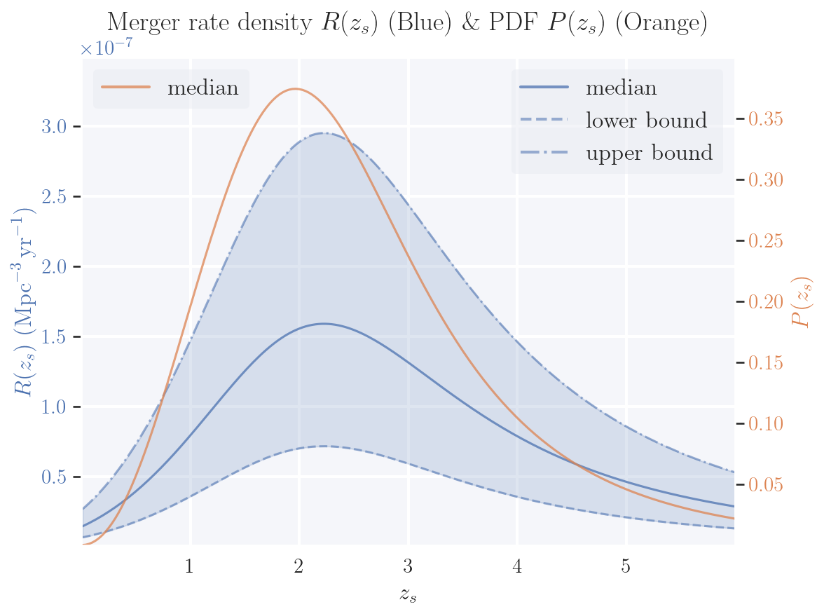
Figure 3 : Redshift evolution of the merger rate density \(R(z_s)\) (blue, left axis) and the probability density function \(P(z_s)\) (orange, right axis) for BBH mergers. Both curves are based on a Madau-Dickinson like model that incorporates time delays and metallicity effects (Ng et al. 2021). The merger rate density is given in \(\mathrm{Mpc}^{-3}\,\mathrm{yr}^{-1}\), with the GWTC-4 local rate \(R_0 = 1.9^{+0.7}_{-0.5} \times 10^{-8}\) and shaded regions showing the uncertainty bounds. The normalized \(P(z_s)\) has no uncertainty band, as the local rate \(R_0\) cancels in its calculation. The rate peaks at \(z_s \approx 2\), reflecting the cosmic star formation history modulated by metallicity (which suppresses BBH formation at low redshift) and time delays. Both \(R(z_s)\) and \(P(z_s)\) decline at higher redshifts, providing insight into gravitational wave detection prospects and the cosmic evolution of compact binaries.

Detection Criterion and SNR Modeling

Assessing detectability requires mapping the population parameters \(\vec{\theta}\) to the detector-frame parameterization used for waveform generation and signal-to-noise ratio SNR evaluation. In particular, the source redshift \(z_s\) is converted to a luminosity distance \(d_L\) using the assumed cosmology, and source-frame component masses are red-shifted to detector-frame masses via \(m_{1,2}=(1+z_s)\,m^{\rm src}_{1,2}\). The resulting detector-frame parameter set may be written as

\[ \begin{split} \vec{\theta}_{\rm det} = \{d_L, m_1, m_2, a_1, a_2, \theta_1, \theta_2, \phi_{12}, \phi_{\rm JL}, \iota, \phi, \psi, {\rm RA}, {\rm Dec}, t_c\} \,, \end{split} \]

where \((\iota,{\rm RA},{\rm Dec},\psi)\) specify the binary orientation and sky location in a geocentric frame. The phase \(\phi\) is the reference orbital phase defined at a chosen reference frequency \(f_{\rm ref}\) (default is \(f_{\rm min}\)), and \(t_c\) is the geocentric coalescence time. Spin degrees of freedom specified by \((a_1,a_2,\theta_1,\theta_2,\phi_{12},\phi_{\rm JL})\) are internally converted to the spin coordinates required by the selected waveform model (for example, Cartesian spin components at \(f_{\rm ref}\)). The detector response is then computed for each interferometer by projecting this common source configuration through detector-specific antenna patterns and time delays, yielding per-detector strains and SNR contributions.

The conditional detection probability \(P({\rm obs}\mid \vec{\theta})\), equivalently \(P({\rm obs}\mid\vec{\theta}_{\rm det})\), is determined by applying a detection threshold \(\rho_{\rm th}\) to the observed SNR \(\rho_{\rm obs}\). In the simplest step-function model, an event is considered detected if its SNR exceeds this threshold. The detection probability is therefore defined as

\[ \begin{split} P({\rm obs} \mid \vec{\theta}) \equiv P_{\rm det} (\vec{\theta}, \rho_{\rm th}) = \Theta[\rho_{\rm obs}(\vec{\theta}) - \rho_{\rm th}] \, , \end{split} \]

where \(\Theta\) is the Heaviside step function. In ler, \(P_{\rm det}\) is evaluated through the gwsnr backend.

To evaluate this criterion, \(\rho_{\rm obs}\) is modeled statistically from the optimal SNR \(\rho_{\rm opt}\). Common approaches treat \(\rho_{\rm obs}\) as either a Gaussian random variable with mean \(\rho_{\rm opt}\) and unit variance (Fishbach et al. 2020; Abbott et al. 2019), or as a non-central chi-squared variable (default in gwsnr and ler) (Essick 2023). The gwsnr package computes \(\rho_{\rm opt}\) efficiently using interpolation or direct inner products, enabling rapid estimation of \(P_{\rm det}\). See the gwsnr documentation for details on detection statistics, optimal SNR, and probability of detection.

Note: \(P_{\rm det}\) in ler is generic and can be used for any detection problem with an SNR-like statistic, including electromagnetic signal detection (e.g., GRB detectability from BNS mergers; More & Phurailatpam 2024).

Complete Expression for GW (unlensed) Event Rate

The observed GW event rate can be expressed as the intrinsic detector-frame rate multiplied by the expectation value of the detection probability over the prior distribution,

\[\begin{split} \begin{split} \frac{\Delta N^{\rm obs}_{\rm U}}{\Delta t} &= {\cal N}_{\rm U} \int_{\vec{\theta}} P({\rm obs} \mid \vec{\theta}) \, P(\vec{\theta}) \, d\vec{\theta} \\ &= {\cal N}_{\rm U} \bigg\langle P({\rm obs} \mid \vec{\theta}) \bigg\rangle_{\vec{\theta} \sim P(\vec{\theta})} \,, \end{split} \end{split}\]

which is evaluated numerically using Monte Carlo integration by drawing samples from \(P(\vec{\theta})\).

Simulation Results

This section reports results generated with the default configuration of the ler package. Although ler supports alternative population prescriptions, including user-defined models, all numbers and figures shown here use the standard settings and assumptions summarized below.

Simulation Settings

All calculations assume a flat \(\Lambda{\rm CDM}\) cosmology with \(H_0 = 70\,{\rm km}\,{\rm s}^{-1}\,{\rm Mpc}^{-1}\), \(\Omega_m = 0.3\), and \(\Omega_\Lambda = 0.7\).

Detection probabilities are evaluated through the gwsnr backend. Waveforms are generated with the IMRPhenomXPHM approximant, and detector responses are computed with a sampling frequency of \(2048\,{\rm Hz}\). The lower frequency cutoff is set to \(f_{\rm low}=20\,{\rm Hz}\) for the LIGO–Virgo–KAGRA network at O4 design sensitivity and \(f_{\rm low}=10\,{\rm Hz}\) for the third-generation (3G) network consisting of Einstein Telescope (ET) and Cosmic Explorer (CE). The detection threshold is set to \(\rho_{\rm th}=10\) for both single detectors and networks. The detector duty cycle is assumed to be 100%.

GW Source Parameter Priors

The prior distributions and parameter ranges used in the event-rate calculations are summarized in Table 1. These choices follow common conventions in gravitational-wave population analyses and are largely consistent with GWTC-3–motivated models, with local rate normalizations taken from the corresponding GWTC-4 reference values quoted below.

Table 1: Prior distributions for GW source parameters

Parameter	Unit	Prior Distribution	Range [Min, Max]	Description
\(z_s\)	-	\(P(z_s)\) derived from Madau- Dickinson SFR	[0, 10]	Source redshift. BBH (Ng et al. 2021, GWTC-4): B=2.57, C=3.36, D=5.83, Median \(R_0 = 1.9 \times 10^{-8}\ \mathrm{Mpc}^{-3}\ \mathrm{yr}^{-1}\). BNS (M&D 2014, GWTC-4): B=2.7, C=2.9, D=5.6 Median \(R_0 = 8.9\times 10^{-8} {\rm Mpc}^{-3}\,{\rm yr}^{-1}\).
\(m^{\rm src}_{1,2}\)	\(M_\odot\)	BBH PowerLaw +Peak BNS Bimodal- Gaussian	BBH [4.98, 112.5] BNS [1.0, 2.3]	Component masses (source-frame). BBH (GWTC-3): \(\alpha\)=3.78, \(\mu_g\)=32.27, \(\sigma_g\)=3.88, \(\lambda_p\)=0.03, \(\delta_m\)=4.8, \(\beta\)=0.81 . BNS (Farr et al. 2020): \(w\)=0.643, \(\mu_L\)=1.352, \(\sigma_L\)=0.08, \(\mu_R\)=1.88, \(\sigma_R\)=0.3 .
\(a_{1,2}\)	-	Uniform	[0, 0.99]	Dimensionless spin magnitudes for primary and secondary objects.
\(\theta_{1,2}\)	rad	Sine	[0, \(\pi\)]	Spin tilt angles relative to \(\vec{L}\) .
\(\phi_{12}\)	rad	Uniform	[0, \(2\pi\)]	Relative azimuthal angle between the two spin vectors about \(\vec{L}\) .
\(\phi_{\rm JL}\)	rad	Uniform	[0, \(2\pi\)]	Precession phase: azimuth of \(\vec{L}\) about \(\vec{J}\) at \(f_{\rm ref}\), measured relative to the projected line of sight (in the plane \(\perp \vec{J}\)).
RA	rad	Uniform	[0, \(2\pi\)]	Right ascension measured in the equatorial plane from the vernal equinox.
Dec	rad	Cosine	[\(-\frac{\pi}{2}\), \(\frac{\pi}{2}\)]	Declination measured from the equatorial plane toward the north celestial pole.
\(\iota\)	rad	Sine	[0, \(\pi\)]	Inclination between the line of sight and \(\vec{L}\) at \(f_{\rm ref}\).
\(\psi\)	rad	Uniform	[0, \(\pi\)]	Polarization angle, measured in the wave plane from the ascending line of nodes to the wave-frame \(x\)-axis
\(\phi\)	rad	Uniform	[0, \(2\pi\)]	Reference orbital phase at the reference frequency \(f_{\rm ref}\).
\(t_c\)	s	Uniform	[0, 1 yr]	Geocentric coalescence time.

Plot Comparison for Detectable and Intrinsic Populations

Selection effects in gravitational-wave observations are illustrated by comparing the intrinsic BBH population to the subset that satisfies the detectability criterion for a given detector network.

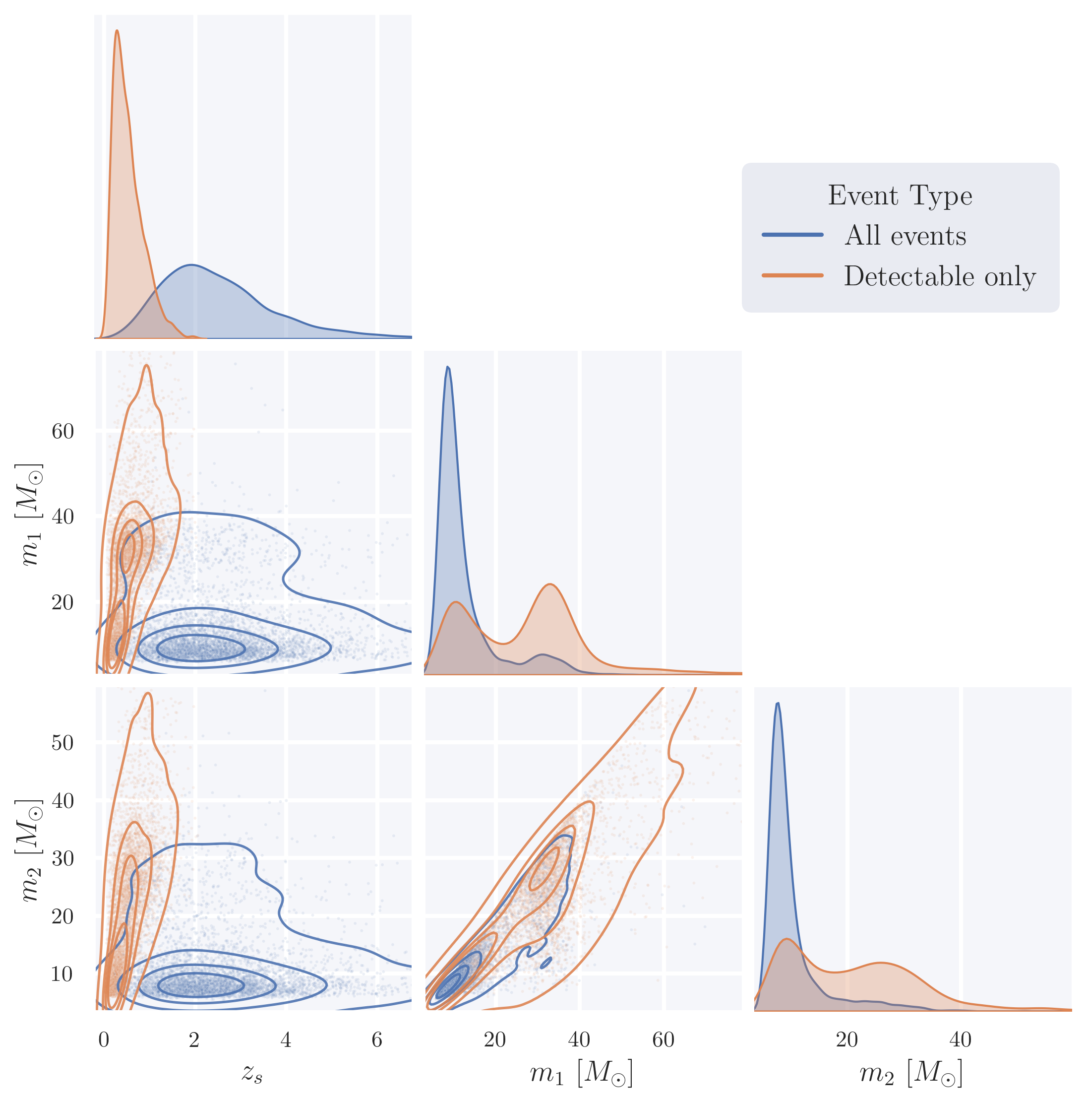
Figure 4: Corner plot comparing the simulated intrinsic BBH population (blue) with the detectable subset (orange) for the LIGO–Virgo–KAGRA network ([‘L1’, ‘H1’, ‘V1’]) at O4 design sensitivity. The population model assumes a Madau–Dickinson–like merger-rate density (see Figure 1) and a PowerLaw+Peak source-frame component-mass distribution; while other parameter distributions follow priors given Table 1. Shown parameters are the source redshift \(z_s\) and component masses in (observed) detector-frame \(\left(m_1, m_2\right)\) and (intrinsic) source-frame \(\left(m^{\rm src}_1=\frac{m_1}{1+z_s}, m^{\rm src}_2=\frac{m_2}{1+z_s}\right)\), in the unit of \(M_\odot\). The detectable subset is biased toward lower redshift and higher masses because these systems typically yield larger network SNR. Orientation effects, which also modulate SNR through the antenna pattern and inclination, are not shown.

Rate Estimates for Different GW Detector Networks

Estimated detectable annual merger rates for BBH and BNS populations are listed below for two detector configurations under the population and detection settings described above.

Detector Configuration	BBH (Pop I–II) Merger Rate (\({\rm yr}^{-1}\))	BNS Merger Rate (\({\rm yr}^{-1}\))	Ratio BBH:BNS
[L1, H1, V1] (O4)	292.7	7.4	39.5
[CE, ET] (3G)	88716	149307	0.6

Notes: O4 design sensitivity and 100% duty cycle are optimistic assumptions for the LIGO–Virgo–KAGRA network. Rates are likely overestimated compared to real observing runs.