Analytical Formulation for Lensed Gravitational Wave Event Rates

Written by Phurailatpam Hemantakumar. Last updated: 2026-02-06.

Overview

This document extends the framework in Analytical Formulation for Gravitational Wave Event Rates to incorporate strong gravitational lensing. The goal is to compute the rate of detectable lensed gravitational-wave (GW) events from compact-binary coalescences (CBCs) by combining the intrinsic merger population with a lens population model, multi-image lensing geometry, and a detection criterion applied to the lensed images. The formulation introduces the optical depth for strong lensing, conditional distributions for source and lens properties given strong lensing, the multi-image caustic cross-section for an EPL+Shear lens model, and the probability of detecting at least two lensed images in a detector network.

Table of Contents

• Introduction

• Parameter-Marginalized Event Rate

• Decomposing the Joint Source–Lens Parameter Distribution

• Source Redshift Distributions of Lensed Events

• Optical Depth

• Lens Redshift Distribution of Lensed Events

• Multi-Image Caustic Cross-Section

• Lens Parameter Distributions of Lensed Events

• Source Position Distribution and Image Properties

• Detection Probability of Lensed Events

• Complete Expression for Lensed Event Rate

• Simulation Results

  • Simulation Settings

  • Lens and source Parameter Priors

  • Plot Comparison for Lensed+Detectable, Lensed and Intrinsic Populations

  • Biases in the inferred GW parameters

  • Time Delays and Magnifications of Detected Lensed Events

  • Rate Estimates and Comparisons

Introduction

The annual rate of detectable strongly lensed GW events, \(\frac{\Delta N^{\rm obs}_{\rm L}}{\Delta t}\), is the expected number of observed lensed CBC mergers per year in a given detector network. It is obtained by scaling the total intrinsic (unlensed) merger rate in the detector frame, \(\frac{\Delta N_{\rm U}}{\Delta t}\), by the joint probability that an intrinsic merger is strongly lensed and detected, denoted \(P({\rm SL,obs})\):

\[ \begin{split} \frac{\Delta N^{\rm obs}_{\rm L}}{\Delta t} = \frac{\Delta N_{\rm U}}{\Delta t}\, P({\rm SL,obs}) \, . \end{split} \]

Using the product rule, \(P({\rm SL,obs})=P({\rm SL})\,P({\rm obs}\mid{\rm SL})\), where \(P({\rm SL})\) is the probability that an intrinsic merger is strongly lensed and \(P({\rm obs}\mid{\rm SL})\) is the conditional probability of detection given strong lensing. This yields

\[ \begin{split} \frac{\Delta N^{\rm obs}_{\rm L}}{\Delta t} = \frac{\Delta N_{\rm U}}{\Delta t}\, P({\rm SL})\, P({\rm obs}\mid{\rm SL}) = {\cal N}_{\rm L}\, P({\rm obs}\mid{\rm SL}) \, , \end{split} \]

where \({\cal N}_{\rm L}\equiv \frac{\Delta N_{\rm U}}{\Delta t}\,P({\rm SL})\) is the total intrinsic rate of strongly lensed mergers, irrespective of detectability.

Parameter-Marginalized Event Rate

The observed lensed event rate is obtained by averaging the detection probability over the unlensed GW parameters \(\vec{\theta}_{\rm U}\), the lens parameters \(\vec{\theta}_{\rm L}\), and the source position \(\vec{\beta}\) within the lens caustic, conditioned on the occurrence of strong lensing. The unlensed GW parameters follow the definitions provided in the unlensed framework, with intrinsic and extrinsic components described in Analytical Formulation for Gravitational Wave Event Rates.

For the Elliptical Power Law with external shear (EPL+Shear) lens model, the lens-parameter vector is

\[ \begin{split} \vec{\theta}_{\rm L}\in \{z_L,\sigma,q,\phi_{\rm rot},\gamma,\gamma_1,\gamma_2\} \, , \end{split} \]

where \(z_L\) is the lens redshift, \(\sigma\) is the velocity dispersion, \(q\) is the projected axis ratio, \(\phi_{\rm rot}\) is the major-axis orientation, \(\gamma\) is the EPL logarithmic density slope, and \((\gamma_1,\gamma_2)\) are the external shear components. The source position on the source plane is \(\vec{\beta}\in\{\beta_x,\beta_y\}\), defined relative to the lens center. The adopted priors are summarized in Lens Parameter Priors.

Given a joint prior distribution \(P(\vec{\theta}_{\rm U},\vec{\theta}_{\rm L},\vec{\beta}\mid{\rm SL})\) conditioned on strong lensing, and a detection probability model \(P({\rm obs}\mid \vec{\theta}_{\rm U},\vec{\theta}_{\rm L},\vec{\beta},{\rm SL})\) for a specific source-lens configuration, the population-averaged detection probability becomes

\[ \begin{split} P({\rm obs}\mid{\rm SL}) = \int P({\rm obs}\mid \vec{\theta}_{\rm U},\vec{\theta}_{\rm L},\vec{\beta},{\rm SL})\, P(\vec{\theta}_{\rm U},\vec{\theta}_{\rm L},\vec{\beta}\mid{\rm SL})\, d\vec{\theta}_{\rm U}\,d\vec{\theta}_{\rm L}\,d\vec{\beta} \, . \end{split} \]

To evaluate this integral with Monte Carlo integration, the unlensed GW parameters are split into the source redshift \(z_s\) and the remaining set \(\vec{\theta}^{*}_{\rm U}\),

\[ \begin{split} \vec{\theta}^{*}_{\rm U}\in \{m_1,m_2,a_1,a_2,\theta_1,\theta_2,\phi_{12},\phi_{\rm JL},\iota,\phi,\psi,t_c, {\rm RA},{\rm Dec}\} \, , \end{split} \]

The lens parameters are split into the lens redshift \(z_L\) and the structural parameters \(\vec{\theta}^{*}_{\rm L}=\{\sigma,q,\phi_{\rm rot},\gamma,\gamma_1,\gamma_2\}\). Under the assumption of isotropic sky locations for sources and lenses, the strong-lensing-conditioned distribution of \((z_s,z_L,\vec{\theta}^{*}_{\rm L})\) is independent of \(({\rm RA},{\rm Dec})\), so that

\[ \begin{split} P(z_s,z_L,\vec{\theta}^{*}_{\rm L}\mid {\rm SL}) \equiv P(z_s,z_L,\vec{\theta}^{*}_{\rm L}\mid {\rm RA},{\rm Dec},{\rm SL}) \, . \end{split} \]

With these decompositions, the lensed detectable rate can be written as the expectation value

\[\begin{split} \begin{split} \frac{\Delta N^{\rm obs}_{\rm L}}{\Delta t} \simeq {\cal N}_{\rm L} \bigg\langle P({\rm obs}\mid \vec{\theta}^{*}_{\rm U},z_s,z_L,\vec{\theta}^{*}_{\rm L},\vec{\beta},{\rm SL}) \bigg\rangle_{\substack{ \vec{\theta}^{*}_{\rm U}\sim P(\vec{\theta}^{*}_{\rm U}) \\ (z_s,z_L,\vec{\theta}^{*}_{\rm L})\sim P(z_s,z_L,\vec{\theta}^{*}_{\rm L}\mid {\rm SL}) \\ \vec{\beta}\sim P(\vec{\beta}\mid z_s,z_L,\vec{\theta}^{*}_{\rm L},{\rm SL}) }} \, . \end{split} \end{split}\]

The expectation value is evaluated by hierarchical sampling from the listed distributions. The sky location \(({\rm RA},{\rm Dec})\) is drawn once from \(P({\rm RA},{\rm Dec})\) and is then held fixed while sampling \((z_s,z_L,\vec{\theta}^{*}_{\rm L})\) and \(\vec{\beta}\) for the same event.

Decomposing the Joint Source–Lens Parameter Distribution

Hierarchical sampling of the lensing configuration is enabled by the chain-rule decomposition, i.e.

\[ \begin{split} P(z_s,z_L,\vec{\theta}^{*}_{\rm L}\mid{\rm SL}) = P(z_s\mid{\rm SL})\,P(z_L\mid z_s,{\rm SL})\,P(\vec{\theta}^{*}_{\rm L}\mid z_L,z_s,{\rm SL}) \, . \end{split} \]

The lens-parameter factor can be expressed using Bayes’ theorem as

\[\begin{split} \begin{split} P(\vec{\theta}^{*}_{\rm L}\mid z_L,z_s,{\rm SL}) &= \frac{P({\rm SL}\mid z_L,z_s,\vec{\theta}^{*}_{\rm L})\,P(\vec{\theta}^{*}_{\rm L}\mid z_L,z_s)}{P({\rm SL}\mid z_L,z_s)} \,,\\ &\propto \sigma_{\rm SL}(z_L,z_s,\vec{\theta}^{*}_{\rm L})\,P(\vec{\theta}^{*}_{\rm L}\mid z_L,z_s) \, , \end{split} \end{split}\]

where \(\sigma_{\rm SL}\) is the strong-lensing angular cross-section (multi-image caustic cross-section in this documentation) and \(P(\vec{\theta}^{*}_{\rm L}\mid z_L,z_s)\) is the prior distribution of lens parameters at fixed redshifts. This factorization motivates drawing \(z_s\) first, then \(z_L\), followed by sampling \(\vec{\theta}^{*}_{\rm L}\) with importance sampling to account for the cross-section weighting.

Source Redshift Distributions of Lensed Events

The redshift distribution of lensed sources differs from the intrinsic distribution because the probability of strong lensing increases with source distance. By Bayes’ theorem,

\[ \begin{split} P(z_s\mid{\rm SL}) = \frac{P({\rm SL}\mid z_s)\,P(z_s)}{P({\rm SL})} \propto P({\rm SL}\mid z_s)\,P(z_s) \, . \end{split} \]

Using the intrinsic unlensed redshift distribution,

\[ \begin{split} P(z_s) = \frac{1}{{\cal N}_{\rm U}}\, \frac{R_{\rm U}(z_s)}{1+z_s}\, \frac{dV_c}{dz_s} \, , \end{split} \]

the lensed-source redshift distribution becomes

\[ \begin{split} P(z_s\mid{\rm SL}) = \frac{1}{{\cal N}_{\rm L}}\, P({\rm SL}\mid z_s)\, \frac{R_{\rm U}(z_s)}{1+z_s}\, \frac{dV_c}{dz_s} \, , \end{split} \]

where \({\cal N}_{\rm U}\) is the total intrinsic merger rate per unit detector-frame time and \({\cal N}_{\rm L}\) is the total intrinsic strongly lensed merger rate per unit detector-frame time. The normalization satisfies

\[ \begin{split} {\cal N}_{\rm L} = {\cal N}_{\rm U}\,P({\rm SL}) = \int P({\rm SL}\mid z_s)\, \frac{R_{\rm U}(z_s)}{1+z_s}\, \frac{dV_c}{dz_s}\,dz_s \, , \end{split} \]

so that \(P({\rm SL})={\cal N}_{\rm L}/{\cal N}_{\rm U}\), which is the fraction of intrinsically occurring mergers that are strongly lensed in the population model. In this work, \(P({\rm SL}\mid z_s)\) is computed for the adopted EPL+Shear lens population as detailed in the subsequent section. Once this probability is determined and the conditional distribution \(P(z_s\mid {\rm SL})\) is established, source redshifts are generated using inverse transform sampling.

Optical Depth

In general radiative-transfer language, the optical depth \(\tau(z_s)\) is the line-of-sight integral of an effective opacity and can be interpreted as the expected number of interactions (absorption, scattering, etc.) experienced by a signal as it propagates through a medium. By direct analogy in strong gravitational lensing, \(\tau(z_s)\) is the expected number of strong-lensing encounters for a source at redshift \(z_s\) under a randomly distributed lens population, where an encounter corresponds to a lens–source configuration in which the source lies inside the multi-image caustic and multiple images form. The optical depth is dimensionless and set by the lens number density and the strong-lensing cross-section. In the low-optical-depth regime \(\tau(z_s)\ll 1\) relevant for galaxy-scale lensing, the probability that the source is strongly lensed satisfies \(P({\rm SL}\mid z_s)\simeq \tau(z_s)\).

A convenient way to derive this relationship is to treat strong-lensing encounters as a Poisson process along the line of sight. If \(\lambda\) denotes the expected number of encounters, the probability of observing exactly \(k\) encounters is given by

\[ \begin{split} P(k) = \frac{\lambda^k e^{-\lambda}}{k!} \, . \end{split} \]

For strong lensing, the Poisson mean \(\lambda\) corresponds to the integrated encounter expectation out to \(z_s\), obtained by summing the angular target size of each potential lens over the lens population along the path. This gives

\[\begin{split} \begin{split} \lambda &= \int ({\rm target\ size}) \times ({\rm number\ density}) \times ({\rm path\ length}) \\ &= \int_{0}^{z_s} \int_{\vec{\theta}^{*}_{\rm L}} \frac{\sigma_{\rm SL}(z_L, z_s, \vec{\theta}^{*}_{\rm L})}{4\pi}\, \frac{d^2N(z_L, \vec{\theta}^{*}_{\rm L})}{dV_c\,d\vec{\theta}^{*}_{\rm L}}\, \frac{dV_c}{dz_L}\, d\vec{\theta}^{*}_{\rm L}\,dz_L \\ &\equiv \tau(z_s) \, . \end{split} \end{split}\]

Geometrically, \(\tau(z_s)\) represents the fraction of the sky covered by the effective strong-lensing cross-sections of all lenses along the line of sight, calculated under the single-lens approximation.

The probability of encountering exactly one strong lens is therefore

\[ \begin{split} P({\rm SL}\mid z_s) = P(k=1\mid \lambda=\tau(z_s)) = \tau(z_s)\,e^{-\tau(z_s)} \, . \end{split} \]

Since \(\tau(z_s)\ll 1\) for galaxy populations on cosmological volumes, this reduces to \(P({\rm SL}\mid z_s)\simeq \tau(z_s)\). A rough estimate using ler shows that typically \(\tau(z_s) \lesssim 0.004\), with the relative difference \(\frac{P({\rm SL} \mid z_s) - \tau(z_s)}{P({\rm SL} \mid z_s)} \times 100 \lesssim 0.4\%\).

In practice, the lens population is often specified by the velocity-dispersion function \(\phi(\sigma,z_L)=\frac{d^2N(z_L,\sigma)}{dV_c\,d\sigma}\). Separating the remaining lens (caustic) shape parameters \(\vec{\theta}^{**}_{\rm L}\) from \(\sigma\), the strong-lensing probability can be written as

\[\begin{split} \begin{split} P({\rm SL}\mid z_s) &\simeq \int_{0}^{z_s}\int_{\sigma,\vec{\theta}^{**}_{\rm L}} \frac{\sigma_{\rm SL}(z_L, z_s, \sigma, \vec{\theta}^{**}_{\rm L})}{4\pi}\, \phi(\sigma,z_L)\\ &\quad\quad\quad\quad \times P(\vec{\theta}^{**}_{\rm L}\mid\sigma)\, \frac{dV_c}{dz_L}\, d\sigma\,d\vec{\theta}^{**}_{\rm L}\,dz_L \, . \end{split} \end{split}\]

It is convenient to introduce the differential optical depth with respect to lens redshift,

\[ \begin{split} P({\rm SL}\mid z_s) \simeq \int_{0}^{z_s} \frac{d\tau}{dz_L}\,dz_L \, , \end{split} \]

where

\[ \begin{split} \frac{d\tau}{dz_L} = \int_{\sigma,\vec{\theta}^{**}_{\rm L}} \frac{\sigma_{\rm SL}(z_L, z_s, \sigma, \vec{\theta}^{**}_{\rm L})}{4\pi}\, \phi(\sigma,z_L)\, P(\vec{\theta}^{**}_{\rm L}\mid\sigma)\, \frac{dV_c}{dz_L}\, d\sigma\,d\vec{\theta}^{**}_{\rm L} \, . \end{split} \]

The function \(d\tau/dz_L\) is used both to evaluate \(\tau(z_s)\) and to construct the lens-redshift distribution \(P(z_L\mid z_s,{\rm SL})\) in the next section.

For the EPL+Shear model, the shape-parameter set is \(\vec{\theta}^{**}_{\rm L}=\{q,\phi_{\rm rot},\gamma,\gamma_1,\gamma_2\}\), and the differential optical depth becomes

\[\begin{split} \begin{split} \frac{d\tau}{dz_L} &= \int_{\sigma,q,\phi_{\rm rot},\gamma,\gamma_1,\gamma_2} \frac{\sigma_{\rm SL}(z_L, \sigma, q,\phi_{\rm rot},\gamma,\gamma_1,\gamma_2)}{4\pi} \phi(\sigma,z_L) \\ & \quad \times P(\gamma_1, \gamma_2) \, P(\gamma) \, P(\phi_{\rm rot}) \, P(q \mid \sigma) \frac{dV_c}{dz_L} \, d\sigma \, dq \, d\phi_{\rm rot} \, d\gamma \, d\gamma_1 \, d\gamma_2\, . \end{split} \end{split}\]

Numerically, this integral is approximated using Monte Carlo integration. To simplify the sampling process, we employ a uniform proposal distribution for the velocity dispersion, \(P_o(\sigma) = 1/\Delta\sigma\), defined over the range of interest \(\Delta\sigma\). Rewriting the integral as an expectation value, the differential optical depth reads

\[\begin{split} \begin{split} \frac{d\tau}{dz_L} = \Delta\sigma \left\langle \frac{\sigma^{\rm EPL}_{\rm SL}}{4\pi}\, \phi(\sigma,z_L)\, \frac{dV_c}{dz_L} \right\rangle_{\substack{ \sigma\sim P_o(\sigma) \\ q\sim P(q\mid\sigma) \\ \phi_{\rm rot}\sim P(\phi_{\rm rot}) \\ \gamma\sim P(\gamma) \\ \gamma_1,\gamma_2\sim P(\gamma_1,\gamma_2) }} \, , \end{split} \end{split}\]

where \(\sigma^{\rm EPL}_{\rm SL}\) denotes the multi-image caustic cross-section for the EPL+Shear model, and each parameter is sampled hierarchically from its respective prior.

Lens Redshift Distribution of Lensed Events

For fixed \(z_s\), the lens-redshift distribution conditioned on the occurance of strong lensing is directly proportional to the differential optical depth, and is given by

\[ \begin{split} P(z_L\mid z_s,{\rm SL}) = \frac{1}{\tau(z_s)}\,\frac{d\tau}{dz_L} \, , \end{split} \]

where the normalization factor is the total optical depth \(\tau(z_s)=\int_{0}^{z_s}(d\tau/dz_L)\,dz_L\). In ler, the differential optical depth \(d\tau/dz_L\) is pre-computed on a grid spanning the relevant redshift space (\(z_L, z_s\)). This grid enables efficient interpolation for inverse-transform sampling of \(z_L\) and allows for rapid evaluation of the strong-lensing probability \(P({\rm SL}\mid z_s)\).

For comparison, the intrinsic redshift distribution of the lens population, without conditioning on strong lensing and independent of any specific background source, is obtained by marginalizing the lens number density over the lens parameters

\[  \begin{split} P(z_L) = \frac{1}{{\cal N}_{z_L}} \int \frac{d^2N(z_L,\vec{\theta}^{*}_{\rm L})}{dV_c\, d\vec{\theta}^{*}_{\rm L}}\, \frac{dV_c}{dz_L}\, d\vec{\theta}^{*}_{\rm L} \, , \end{split} \]

where \({\cal N}_{z_L}\) is a normalization constant.

The impact of the optical depth on the source redshift distributions of the lensed events is illustrated in Figure 1.

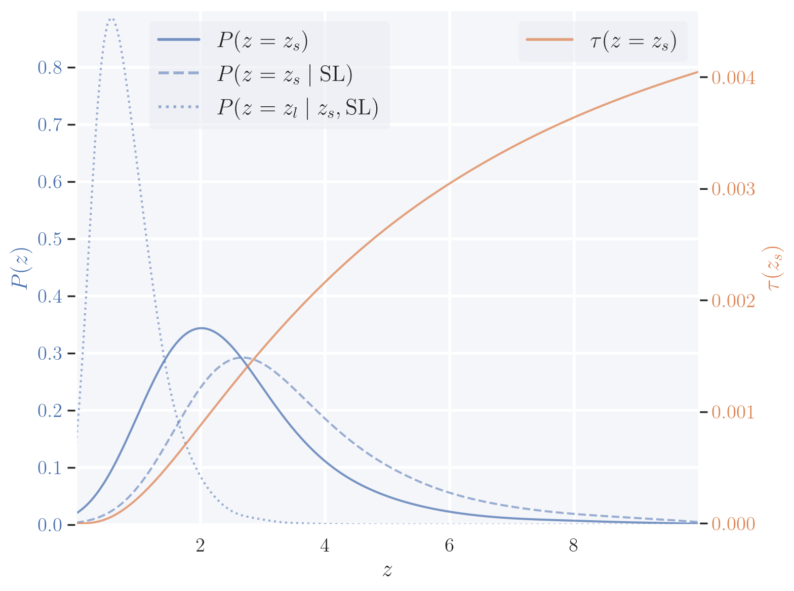
Figure 1: Redshift distributions (blue, left axis) for the intrinsic source population \(P(z=z_s)\), the lensed-source population \(P(z=z_s\mid{\rm SL})\), and the conditional lens distribution \(P(z=z_L\mid z_s,{\rm SL})\), shown together with the optical depth \(\tau(z=z_s)\) (orange, right axis), which quantifies the strong-lensing probability for a source at redshift \(z_s\) in the low-optical-depth regime. The intrinsic \(P(z_s)\) follows the unlensed merger-rate model, while \(P(z_s\mid{\rm SL})\) is obtained by reweighting the intrinsic population by the lensing probability, \(P(z_s\mid{\rm SL})\propto \tau(z_s)\,P(z_s)\), implemented via rejection sampling using \(\tau(z_s)\). For each lensed source, the lens redshift is drawn from \(0<z_L<z_s\) with a density proportional to \(\frac{d\tau}{dz_L}\), so that \(P(z_L\mid z_s,{\rm SL})\) traces where along the line of sight the lenses that produce strong lensing are most likely to occur. Since \(\tau(z_s)\) increases with redshift, strong lensing preferentially selects more distant sources and shifts \(P(z_s\mid{\rm SL})\) to higher redshift relative to \(P(z_s)\), while \(P(z_L\mid z_s,{\rm SL})\) describes the redshift distribution of the lenses responsible for that lensed-source population.

Multi-Image Caustic Cross-Section

The strong-lensing condition is satisfied when a source resides within the multi-image caustic region in the source plane, which encompasses the area enclosed by both the double and diamond (quad) caustics (see Figure 2), thereby producing multiple images. The angular area of this region is defined as the multi-image caustic cross-section, \(\sigma_{\rm SL}\) (denoted as \(\sigma^{\rm EPL}_{\rm SL}\) for the EPL+Shear model). The probability of strong lensing for a specific configuration is the ratio of this cross-section to the total sky area

\[ \begin{split} P({\rm SL}\mid z_L, z_s, \vec{\theta}^{*}_{\rm L}) = \frac{\sigma_{\rm SL}}{4\pi} \, . \end{split} \]

Direct evaluation of \(\sigma_{\rm SL}\) by tracing caustics with lenstronomy is computationally expensive. In ler, \(\sigma^{\rm EPL}_{\rm SL}\) is therefore precomputed on the grid of lens (caustic) shape parameters \(\vec{\theta}^{**}_{\rm L}\in \{q,\phi_{\rm rot},\gamma,\gamma_1,\gamma_2\}\) at unit Einstein radius \(\theta_{\rm E}=1\), and interpolated during sampling. For arbitrary \((\sigma,z_L,z_s)\), the Einstein radius is

\[ \begin{split} \theta_{\rm E} = 4\pi\left(\frac{\sigma}{c}\right)^2 \frac{D_{LS}(z_L,z_s)}{D_S(z_s)} \, , \end{split} \]

where \(D_{LS}\) and \(D_S\) are angular-diameter distances.

The cross-section is then rescaled from the \(\theta_{\rm E}=1\) values using the calibrated relation

\[\begin{split} \begin{split} \sigma^{\rm EPL}_{\rm SL}(\theta_{\rm E}, q, \phi_{\rm rot}, \gamma, \gamma_1, \gamma_2) &= \sigma^{\rm EPL}_{\rm SL}(1, q, \phi_{\rm rot}, \gamma, \gamma_1, \gamma_2) \\ &\quad\times \left({\rm intercept} + {\rm slope}\,\pi\,\theta_{\rm E}^2\right) \, , \end{split} \end{split}\]

where \({\rm intercept}\) and \({\rm slope}\) are precomputed constants. This interpolation and rescaling scheme accelerates cross-section evaluation and, consequently, the computation of \(\frac{d\tau}{dz_L}\).

Going forward, I simply use the term ‘cross-section’ to refer to \(\sigma_{\rm SL}\) or \(\sigma^{\rm EPL}_{\rm SL}\).

Lens Parameter Distributions of Lensed Events

For a fixed redshift pair \((z_L,z_s)\), the conditional distribution of lens parameters \(P(\vec{\theta}^{*}_{\rm L}\mid z_L,z_s,{\rm SL})\) is determined by weighting the intrinsic lens population with the strong-lensing cross-section \(\sigma^{\rm EPL}_{\rm SL}(z_L,z_s,\vec{\theta}^{*}_{\rm L})\). For the EPL+Shear model, this target distribution is expressed as

\[\begin{split} \begin{split} &P(\sigma, q, \phi_{\rm rot}, \gamma, \gamma_1, \gamma_2 \mid z_L, z_s, {\rm SL})\\ &\quad \propto P({\rm SL}\mid z_L, z_s, \sigma, q, \phi_{\rm rot}, \gamma, \gamma_1, \gamma_2) \, P(\gamma_1, \gamma_2) \, P(\gamma) \, P(\phi_{\rm rot}) \, P(q \mid \sigma) \, P(\sigma \mid z_L) \\ &\quad \propto \frac{\sigma^{\rm EPL}_{\rm SL}}{4\pi} \, P(\gamma_1, \gamma_2) \, P(\gamma) \, P(\phi_{\rm rot}) \, P(q \mid \sigma) \, P(\sigma \mid z_L) \, . \end{split} \end{split}\]

Direct rejection sampling from the intrinsic distribution \(P(\sigma\mid z_L)\) is computationally inefficient because the lensing cross-section \(\sigma^{\rm EPL}_{\rm SL}\) scales roughly as \(\sigma^4\), heavily favoring high-mass lenses that are exponentially rare in the intrinsic population. Furthermore, the lack of a strict analytical maximum for the cross-section complicates the definition of a rejection envelope.

To address these challenges, ler employs importance sampling. A proposal distribution \(P_o(\sigma)\), typically chosen to be uniform over \([\sigma_{\min},\sigma_{\max}]\), is introduced to rewrite the target density. By defining the intrinsic distribution \(P(\sigma \mid z_L)\) as the normalized velocity dispersion function \(\phi(\sigma, z_L)/\int \phi(\sigma', z_L) d\sigma'\), the target distribution becomes

\[\begin{split} \begin{split} &P(\sigma, q, \phi_{\rm rot}, \gamma, \gamma_1, \gamma_2 \mid z_L, z_s, {\rm SL})\\ &\quad \propto \left[\frac{ \sigma^{\rm EPL}_{\rm SL}\, P(\sigma \mid z_L)}{4\pi\,P_o(\sigma)}\right] P(\gamma_1, \gamma_2) \, P(\gamma) \, P(\phi_{\rm rot}) \, P(q \mid \sigma) \, P_o(\sigma) \\ &\quad = \frac{1}{{\cal W}(z_L)} \left[\frac{ \sigma^{\rm EPL}_{\rm SL}\, \phi(\sigma, z_L)}{P_o(\sigma)}\right] P(\gamma_1, \gamma_2) \, P(\gamma) \, P(\phi_{\rm rot}) \, P(q \mid \sigma) \, P_o(\sigma) \, . \end{split} \end{split}\]

In this formulation, constant factors including \(4\pi\) and the normalization of the intrinsic velocity dispersion function are absorbed into the overall normalization constant \({\cal W}(z_L)\). The term in the square brackets represents the unnormalized importance weight required to convert samples from the proposal distribution into samples from the cross-section-weighted target distribution.

Computationally, this is implemented by generating a candidate batch of size \(N_{\rm prop}\) (defaulting to 200 in ler) for each \((z_L, z_s)\) pair. The velocity dispersion \(\sigma_i\) is drawn from the proposal \(P_o(\sigma)\), while the remaining shape parameters are sampled directly from their intrinsic priors. Each candidate in the batch is assigned a normalized importance weight

\[ \begin{split} w_i(\sigma_i, q_i, \phi_{{\rm rot},i}, \gamma_i, \gamma_{1,i}, \gamma_{2,i};z_L,z_s)=\frac{1}{{\cal W}(z_L)}\,\frac{\sigma^{\rm EPL}_{{\rm SL}, i}\,\phi(\sigma_i, z_L)}{P_o(\sigma_i)} \, , \end{split} \]

where the batch normalization constant is defined as the sum of the unnormalized weights

\[ \begin{split} {\cal W}(z_L)=\sum_{i=1}^{N_{\rm prop}}\frac{\sigma^{\rm EPL}_{{\rm SL}, i}\,\phi(\sigma_i, z_L)}{P_o(\sigma_i)} \, . \end{split} \]

A final lens configuration is selected from this batch by resampling with probabilities proportional to \(w_i\), ensuring the final parameter set accurately reflects the properties of the strongly lensed population.

Source Position Distribution and Image Properties

Given \((z_s,z_L,\vec{\theta}^{*}_{\rm L})\), the source position \(\vec{\beta}\) is sampled uniformly within the multi-image caustic so that each draw produces multiple images. The lens equation is solved with lenstronomy to obtain the image positions \(\vec{\theta}_i\in \{\theta_{x,i},\theta_{y,i}\}\), magnifications \(\mu_i\), and arrival-time delays \(t_i\). These quantities are initially computed at \(\theta_{\rm E}=1\) and then rescaled to physical units using the system’s \(\theta_{\rm E}\).

Each image is assigned a Morse index \(n_i\in\{0,1/2,1\}\) corresponding to minima (Type I), saddles (Type II), and maxima (Type III), respectively. Type III images are typically highly demagnified and are neglected in the detectability criterion adopted here. Lensing modifies the observed GW parameters for each image \(i\) as follows

\[\begin{split} \begin{split} d_L &\rightarrow \frac{d_L(z_s)}{\sqrt{\lvert\mu_i\rvert}}\,, \\ \phi_c &\rightarrow \phi_c - n_i\pi\,, \\ t_c &\rightarrow t_c + t_i \, , \\ {\rm RA} &\rightarrow {\rm RA} + \frac{\theta_{x,i}-\beta_x}{\cos({\rm Dec})}\,, \\ {\rm Dec} &\rightarrow {\rm Dec} + (\theta_{y,i}-\beta_y)\,, \\ \end{split} \end{split}\]

while the other extrinsic and intrinsic parameters are unchanged from the unlensed values, including the detector-frame component masses \(\left(m_1 \, (1+z_s),m_2 \, (1+z_s)\right)\). The sky-location offsets associated with \(\vec{\theta}_i-\vec{\beta}\) are typically negligible for current GW detector networks and have no impact on SNR. Detectability is therefore evaluated by computing the SNR for each image using the modified GW pararameters \(\vec{\theta}_{{\rm GW},i}\), as described in the next section.

Note: The lens-centre coordinates in the sky is given by \(\left\{ {\rm RA} - \frac{\beta_x}{\cos({\rm Dec})}, {\rm Dec} - \beta_y \right\}\).

An illustrative example of a multi-image configuration for an EPL+Shear lens is shown in Figure 2, where the source is located near a fold caustic boundary, resulting in four images with two highly magnified ones. The lens parameters are chosen to produce a typical caustic structure with an outer double-image caustic and an inner diamond-shaped quad-image caustic. The image properties (type, magnification) are determined by the source position relative to these caustics and the lens parameters that govern their shape and size.

Figure 2: Interactive multi-image configuration for an EPL+Shear lens model, displaying the outer double-image caustic (orange, dashed) and the inner quad-image (diamond) caustic (green, solid) in the source plane. The Einstein ring (blue, dotted) serves as the angular scale reference, with \(\theta_E(z_s=3.0, z_L=0.8, \sigma=160,{\rm km/s}) \approx 2 \times 10^{-6}\) rad. The default lens geometry is defined by an axis ratio \(q=0.6\), orientation angle \(\phi=0.52\) rad, mass density slope \(\gamma=1.84\), and external shear components \(\gamma_1=\gamma_2=-0.05\); all parameters are adjustable via the sliders. A source placed at \((\beta_x, \beta_y) = (-0.25, 0.04)\) lies inside the diamond caustic near a fold boundary, generating four lensed images (stars). These are labeled by index \(i\) (ordered by arrival time, where \(i=1\) arrives first), image type, and absolute magnification \(|\mu_i|\). The caustic structure is governed by the lens parameters: \(q\) controls ellipticity, \(\phi\) sets the counter-clockwise orientation relative to the \(x\)-axis, increasing \(\gamma\) causes the outer caustic to expand while the inner diamond caustic shrinks, and the shear components introduce skewness and rotation. In this default configuration the source lies near a caustic fold, producing high-magnification images that can significantly enhance the detectability of gravitational lensing systems. A Python-based version of this interactive demonstration, which also includes time-delay calculations, is available in the Google Colab Example Notebook.

Detection Probability of Lensed Events

For a specific lensed configuration, the detection probability is determined by the detectability of its images. The signal-to-noise ratio (SNR), \(\rho(\vec{\theta}_{{\rm GW},i})\), is computed for each image using the modified GW parameters. An event is considered detected if at least two images meet the detection criterion. The probability is therefore a binary condition

\[ \begin{split} &P({\rm obs} \mid \vec{\theta}^*_{\rm U}, z_s, \vec{\theta_{\rm L}}, \vec{\beta}, {\rm SL}) = \Theta\left[\left(\sum_i P_{\rm det}(\vec{\theta}_{{\rm GW},i}, \rho_{\rm th}) \right) - 2\right] \, , \end{split} \]

where \(\Theta\) is the Heaviside step function and the sum is over all images \(i\). In the simplest step-function model, the individual image detection probability is defined as

\[ \begin{split} P_{\rm det} (\vec{\theta}, \rho_{\rm th}) = \Theta[\rho(\vec{\theta}_{{\rm GW},i}) - \rho_{\rm th}] \, , \end{split} \]

and in ler, it is estimated using the gwsnr package.

Complete Expression for Lensed Event Rate

Summarizing the derivation steps, the annual rate of detectable strongly lensed GW events is given by

\[\begin{split} \begin{split} \frac{\Delta N^{\rm obs}_{\rm L}}{\Delta t} &= {\cal N}_{\rm L} \bigg\langle P({\rm obs}\mid \vec{\theta}^{*}_{\rm U}, z_s, \vec{\theta}_{\rm L}, \vec{\beta}, {\rm SL}) \bigg\rangle_{\substack{ \vec{\theta}^{*}_{\rm U}\sim P(\vec{\theta}^{*}_{\rm U}) \\ z_s \sim P(z_s \mid {\rm SL}) \\ z_L \sim P(z_L \mid z_s, {\rm SL}) \\ \vec{\theta}^{*}_{\rm L} \sim P(\vec{\theta}^{*}_{\rm L} \mid z_L, z_s, {\rm SL}) \\ \vec{\beta} \sim P(\vec{\beta} \mid z_s, \vec{\theta}_{\rm L}, {\rm SL}) }} \, . \end{split} \end{split}\]

The computational procedure for evaluating the rate via Monte Carlo integration is summarized as follows:

1. Intrinsic GW Parameters: Sample the unlensed GW parameters \(\vec{\theta}^{*}_{\rm U}\) from their intrinsic priors \(P(\vec{\theta}^{*}_{\rm U})\).

2. Lensed Source Redshift: Sample the source redshift \(z_s\) via inverse-transform sampling from the lensed distribution \(P(z_s \mid {\rm SL})\), which is derived from the intrinsic redshift distribution \(P(z_s)\) and the precomputed optical depth \(\tau(z_s)\).

3. Lens Redshift: Conditioned on the sampled \(z_s\), sample the lens redshift \(z_L\) via inverse-transform sampling from the distribution \(P(z_L \mid z_s, {\rm SL})\), which is determined numerically from the differential optical depth \(d\tau/dz_L\).

4. Lens Properties: Conditioned on \((z_s, z_L)\), generate a candidate batch of lens parameters \(\{ \vec{\theta}^{*}_{{\rm L},i} \}_{i=1}^{N_{\rm prop}}\). Draw shape parameters \(\vec{\theta}^{**}_{{\rm L},i}\) from their intrinsic priors \(P(\vec{\theta}^{**}_{\rm L} \mid z_L, z_s)\) and velocity dispersions \(\sigma_i\) from a uniform proposal \(P_o(\sigma)\). Select a single final configuration from this batch using importance sampling with normalized weights \(w_i = \frac{1}{{\cal W}(z_L)}\frac{\sigma^{\rm EPL}_{{\rm SL},i}\,\phi(\sigma_i\mid z_L)}{P_o(\sigma_i)}\), where \({\cal W}(z_L)\) ensures \(\sum_i w_i=1\).

5. Source Position: Sample the source position \(\vec{\beta}\) uniformly within the multi-image caustic region defined by the selected lens parameters, calculated at a reference Einstein radius \(\theta_{\rm E}=1\).

6. Image Properties: Solve the lens equation to obtain the normalized image positions \(\vec{\theta}_i\), magnifications \(\mu_i\), and time delays \(t_i\). Rescale the geometric parameters \(\vec{\beta}\), \(\vec{\theta}_i\), and \(t_i\) to physical units using the physical Einstein radius \(\theta_{\rm E}(\sigma, z_L, z_s)\).

7. Observed GW Parameters: Construct the observed parameters \(\vec{\theta}_{{\rm GW},i}\) for each image by applying lensing transformations (magnification, time delay, Morse phase shift and source position offsets) to the unlensed parameters \(\vec{\theta}^{*}_{\rm U}\).

8. Detection Criteria: Compute the SNR \(\rho(\vec{\theta}_{{\rm GW},i})\) for each image. An event is classified as detected if at least two images satisfy the detection threshold, i.e., \(P({\rm obs}\mid \vec{\theta}^{*}_{\rm U}, z_s, \vec{\theta}_{\rm L}, \vec{\beta}, {\rm SL})=1\) if \(\sum_i \rho(\vec{\theta}_{{\rm GW},i})\geq 2\) otherwise \(0\).

9. Rate Estimation: Estimate the final observable rate by averaging the detection probability \(P({\rm obs}\mid \vec{\theta}^{*}_{\rm U}, z_s, \vec{\theta}_{\rm L}, \vec{\beta}, {\rm SL})\) over a large ensemble (typically \(\gtrsim 10^6\)) of parameter sets \(\{\vec{\theta}^{*}_{\rm U}, z_s, \vec{\theta}_{\rm L}, \vec{\beta} \}\) and scaling the result by the total lensed rate \({\cal N}_{\rm L}\).

The specific parameter priors and their functional forms are detailed below.

Simulation Results

This section details the results regarding strong gravitational-wave lensing generated using the default configuration of the ler package. These results are compared against unlensed events. While ler accommodates alternative population prescriptions and user-defined models, the subsequent calculations rely on standard settings and assumptions.

Simulation Settings

The cosmological framework assumes a flat \(\Lambda{\rm CDM}\) model with \(H_0 = 70\,{\rm km}\,{\rm s}^{-1}\,{\rm Mpc}^{-1}\), \(\Omega_m = 0.3\), and \(\Omega_\Lambda = 0.7\). Detection probabilities are computed via the gwsnr backend. Waveforms are generated using the IMRPhenomXPHM approximant. Detector responses are evaluated at a sampling frequency of \(2048\,{\rm Hz}\) with a lower frequency cutoff of \(f_{\rm low}=20\,{\rm Hz}\) for the LIGO–Virgo–KAGRA network at O4 design sensitivity. The signal-to-noise ratio detection threshold is established at \(\rho_{\rm th}=10\) for the network, assuming a complete 100% detector duty cycle.

Lens and source Parameter Priors

GW Source Parameter Priors are kept the same as in the section GW Source Parameter Priors of Analytical Formulation for Gravitational Wave Event Rates. The lens prior distributions and parameter ranges used in the event-rate calculations are summarized in Table 1, Table 2 and Table 3. These choices follows common conventions such as GW population forllowing GWTC-3–motivated models for source and SDSS and SLACS observations of galaxy populations.

Gravitational-wave source parameter priors align with those specified in the unlensed framework. The lens prior distributions and parameter ranges employed in the event-rate calculations follow standard conventions based on GWTC-3 motivated source models alongside SDSS and SLACS galaxy observations. Table 1, Table 2, and Table 3 summarize these parameters. The source and lens redshifts are drawn from distributions conditioned on the occurrence of strong lensing. The optical depth \(\tau(z_s)\) and the differential optical depth \(d\tau/dz_L\) are pre-computed using the adopted EPL+Shear lens population and cosmology.

Table 1: Prior distributions for source and lens redshifts.

Parameter	Unit	Prior Distribution	Range [Min, Max]	Description
\(z_s\)	-	\(P(z_s\mid {\rm SL})\) \(\propto \tau(z_s)\,P(z_s)\)	[0, 10]	Source redshift conditioned on \({\rm SL}\)
\(z_L\)	-	\(P(z_L\mid z_s,{\rm SL})\) \(\propto \frac{d\tau}{dz_L}\)	[0, \(z_s\)]	Lens redshift conditioned on \(z_s\) and \({\rm SL}\)

Lens parameter priors are listed below. Shape parameters assume a local flat coordinate system, with thin lens approximation, where the x-axis and the y-axis align with sky coordinates right ascension and declination respectively.

Table 2: Prior distributions for lens parameters

Parameter	Unit	Prior Distribution	Range [Min, Max]	Description
\(\sigma\)	km/s	Proposed prior Uniform Physical prior \(P(\sigma\mid z_L)\propto\) \(\phi(\sigma, z_L)\)	[100, 400]	Velocity dispersion. Proposed prior : Used for importance sampling and computing \(\frac{d\tau}{dz_L}\). Physical prior : Based on the velocity dispersion function \(\phi(\sigma, z_L)\) (Oguri et al. 2018; SDSS+Illustris). \(\alpha\)=0.94, \(\beta\)=1.85, \(\phi_*\)=2.099x10\(^{-2}\)x(h/0.7)\(^{3}\) Mpc\(^{-3}\), \(\sigma_*\)=113.78 km/s. It is used to calculate importance weights and \(d\tau/dz_L\), rather than for direct sampling.
\(q\)	-	\(P(q\mid \sigma)\) Rayleigh distribution	[0.2, 1.0]	Projected axis ratio, conditioned on \(\sigma\) (Collett et al. 2015; SDSS).
\(\phi_{\rm rot}\)	rad	Uniform	[0, \(\pi\)]	Lens orientation angle, measured counter-clockwise from the x-axis.
\(\gamma\)	-	Normal	-	Density profile slope (Sonnenfeld et al. 2024; SLACS). Mean: 2.0, Std: 0.1
\(\gamma_1, \gamma_2\)	-	Normal	-	External shear (Collett et al. 2015; SDSS). x and y components. Mean: 0.0, Std: 0.05

Source positions \(\beta\) are defined in a local flat coordinate system matching the orientation of the shape parameters.

Table 3: Prior distributions for source position

Parameter	Unit	Prior Distribution	Description
\(\beta_x\)	\(\theta_{\rm E}\)	Uniform within multi-image caustic	x-component of source position from lens center
\(\beta_y\)	\(\theta_{\rm E}\)	Uniform within multi-image caustic	y-component of source position from lens center

Plot Comparison for Lensed+Detectable, Lensed and Intrinsic Populations

Selection effects inherent in lensed gravitational-wave observations become apparent when comparing the intrinsic binary black hole population to the subsets satisfying the strong-lensing condition and the detection criteria. The first subset is denoted as the strongly lensed population, and the second is referred to as the detectable strongly lensed population.

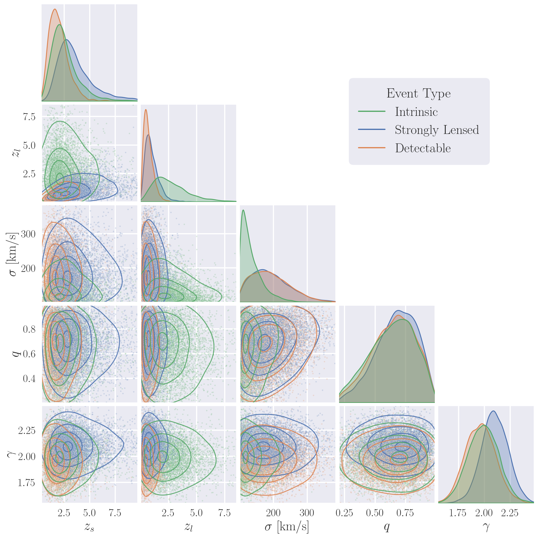
Figure 4: Kernel density estimate corner plot with 10, 40, 68, and 95 percent contour levels comparing parameter distributions for simulated intrinsic events (green), strongly lensed events (SL, blue), and strongly lensed events that also satisfy the detection criterion (SL+obs, orange), shown for the source redshift \(z_s\), lens redshift \(z_L\), lens velocity dispersion \(\sigma\), projected axis ratio \(q\), and EPL density slope \(\gamma\); other lens parameters are omitted because their distributions show no significant changes under the SL and SL+obs selections. The intrinsic source population follows the unlensed merger-rate model, adopting a Madau–Dickinson–like prescription with time-delay and metallicity effects (see Figure 1) and standard GW-source priors as in the unlensed framework, while the intrinsic lens population is described by the velocity-dispersion function \(\phi(\sigma,z_L)\) from Oguri et al. (2018), with SDSS-based local calibration and redshift evolution informed by Illustris (Torrey et al. 2015), and with axis ratios drawn from a \(\sigma\)-conditioned Rayleigh model (Collett 2015), together with the remaining shape priors in Table 2. Strong lensing acts primarily through the optical depth and the lensing cross-section, set by the angular area of the multi-image caustic, so it preferentially selects higher-\(z_s\) sources where the optical depth is larger and favors higher-\(\sigma\) lenses because the cross-section scales steeply with Einstein radius, approximately as \(\sigma^4\), while the conditional lens-redshift distribution peaks at intermediate redshifts \(0<z_L<z_s\) where lensing efficiency is highest. The detectability requirement introduces a secondary selection layer. Once a source lies inside the multi-image caustic, the probability of inclusion in SL+obs increases with the number of images and their magnifications, and the largest magnifications typically arise for sources near caustic boundaries, particularly within the quad caustic, which can boost the SNR and extend the detection horizon, making larger quad-caustic regions relative to the double-caustic region more favorable. Consistent with these trends, the SL population shows a preference for steeper density profiles (higher \(\gamma\)) and rounder lenses (higher \(q\)) that generally yield larger caustic areas, whereas the SL+obs subset is biased toward lower redshift by SNR limitations and shows a mild shift toward more elliptical lenses (lower \(q\)) and slightly shallower slopes (lower \(\gamma\)) relative to SL because these configurations can increase the chances of highly magnified multi-image signals (including quads). The figure therefore demonstrates that strong lensing and detectability together imprint coupled selection effects on \((z_s,z_L,\sigma,q,\gamma)\) that must be modeled self-consistently when simulating observed lensed events and interpreting inferred source and lens properties, and an interactive illustration of how \((q,\phi,\gamma,\gamma_1,\gamma_2)\) reshape caustics and image magnifications is provided in the example notebook.

Biases in the inferred GW parameters

When a strongly lensed gravitational wave is detected without being identified as such, parameter estimation proceeds using standard unlensed waveform templates. Since lensing magnifies the signal, the effective luminosity distance is artificially decreased. Under the assumption of standard cosmology, this shorter distance is interpreted as a lower source redshift. The source-frame masses, obtained by de-redshifting the detector-frame masses using this underestimated redshift, are consequently biased upward. This systematic shift is referred to as magnification bias.

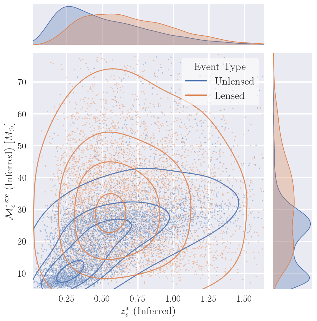
Figure 5: Joint kernel density estimate (KDE) with 10, 40, 68, and 95 percent contour levels and marginal distributions comparing the inferred source redshift \(z^*_s\) and inferred source-frame chirp mass \({\cal M}_c^{* \, {\rm src}}\) for the detectable unlensed (blue) and lensed (orange) populations. Number of data points should not be interpreted as relative rates. While the unlensed parameters reflect the true source properties, the inferred parameters for lensed events are systematically biased by magnification. The inferred redshift \(z^*_s\) is derived from the effective luminosity distance \(d_{L}^{\rm eff} = d_{L} / \sqrt{|\mu|}\), which subsequently affects the source-frame mass reconstruction via \({\cal M}_c^{* \, {\rm src}} = {\cal M}_c / (1+z^*_s)\), where \({\cal M}_c\) is the detector-frame chirp mass. Consequently, the lensed population exhibits a distinct shift toward higher inferred redshifts—though these still underestimate the true source redshifts of lensed events—and significantly higher inferred chirp masses relative to the unlensed population. This magnification bias demonstrates that unrecognized lensed events can contaminate the observed catalog by mimicking heavy binary black hole mergers and appearing as high-mass outliers; however, given the low expected rate of lensed events relative to unlensed ones (\(\approx\) 1:3000 at O4 design sensitivity), this contamination is unlikely to significantly skew population studies or cosmological inferences even if unaccounted for.

Time Delays and Magnifications of Detected Lensed Events

Strong gravitational lensing produces multiple copies of the same transient signal arriving at the detector at different times and with varying amplitudes. The distinct arrival times define a time delay between images, while the relative amplitudes yield a magnification ratio. Comparing these pairwise observables provides a simple discriminative tool for distinguishing genuine lensed image pairs from random coincidences of independent unlensed events.

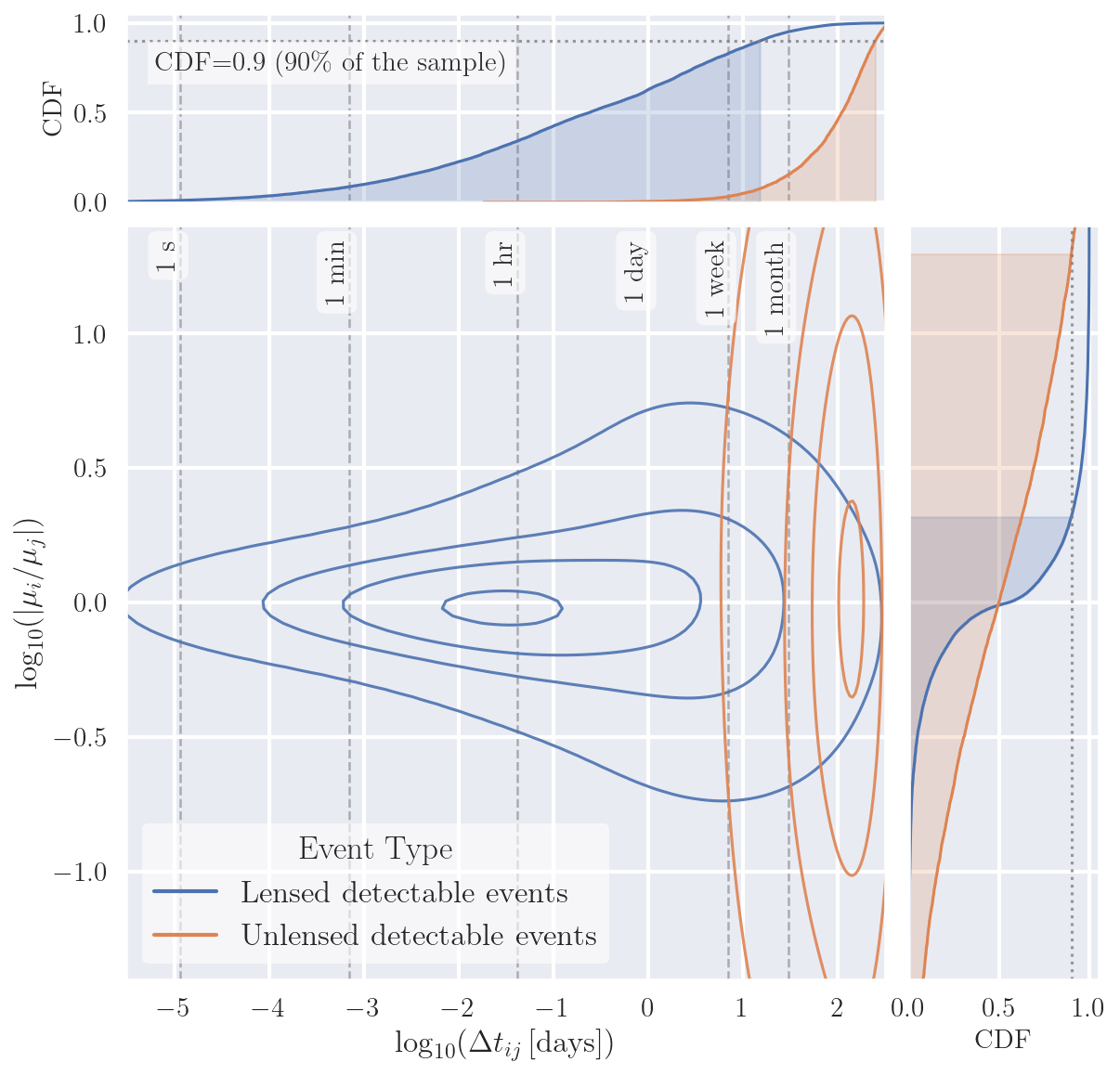
Figure 6: Joint kernel density estimate in the plane of pairwise time-delay difference \(\log_{10}(\Delta t_{ij})\) and relative magnification \(\log_{10}(|\mu_i/\mu_j|)\), comparing pairs of detected images from strongly lensed events (blue) to pairs of randomly chosen detected unlensed events (orange), with the corresponding marginal empirical cumulative distribution functions (CDFs) shown in the top and right panels. For lensed systems, \(\Delta t_{ij}\) is the arrival-time delay between the \(i\)th and \(j\)th (detected) images of the same source (in days, with \(i<j\)), and \(\mu_i\) and \(\mu_j\) are the signed lensing magnifications; the ratio can be expressed in terms of effective luminosity distances as \(|\mu_i / \mu_j|=(d^{\rm eff}_{L,i}/d^{\rm eff}_{L,j})^2\) with \(d^{\rm eff}_{L}=d_L/\sqrt{|\mu|}\). The unlensed comparison represents the distribution of time separations and luminosity-distance ratios for unrelated (detected) events, rather than multiple images of a single source. The lensed population is concentrated at shorter delays and closer-to-unity magnification ratios, with 90% of pairs satisfying \(\Delta t{ij}<15.09\) days (equivalently \(\log_{10}(\Delta t_{ij})<1.179\)) and \(|\mu_i/\mu_j|<2.081\) (equivalently \(\log_{10}(|\mu_i/\mu_j|)<0.318\)), whereas the unlensed pairs exhibit a much broader distributions with 90% satisfying \(\Delta t_{ij}<244.28\) days (\(\log_{10}(\Delta t_{ij})<2.388\)) and \(|\mu_i/\mu_j|<17.282\) (\(\log_{10}(|\mu_i/\mu_j|)<1.238\)), including very small ratios arising from widely different distances. This separation motivates using \((\Delta t_{ij},|\mu_i/\mu_j|)\) as a diagnostic for lensing candidates identification, since pairs with small \(\Delta t_{ij}\) and \(|\mu_i/\mu_j|\simeq 1\) are more consistent with being multiple images of the same lensed event than with being unrelated detections (Janquart et al. 2023)

Rate Estimates and Comparisons

Estimated detectable annual merger rates for BBH (Pop I–II) populations are listed below.

Detector Configuration	Unlensed Merger Rate (\({\rm yr}^{-1}\))	Lensed Merger Rate (\({\rm yr}^{-1}\))	Ratio Unlensed:Lensed
[L1, H1, V1] (O4)	299.56	0.10	2996:1